This is Deeplearning2C. It's a project for generate an application for Android, Iphone, Linux, Windows and Mac OS X, that can generate a deep neural network in a .c file and .m file after being trained with Deeplearning4J.
I have been using mimimal dependencies and liberaries. These are the the following dependencies I have been using:
- Deeplearning4J
- GluonHQ JavaFX for Android & Iphone development
- Lombok
- Logback-classic
Let's say that you want to implement an deep neural network that are trained for classification for animals or other visible things. You want to implement it into a microcontroller such as STM32, PIC, AVR. Then this application can be used to generate a deep neural network in C code.
Here is an example when I run the IRIS example with iris.csv data file. You can download it from here:
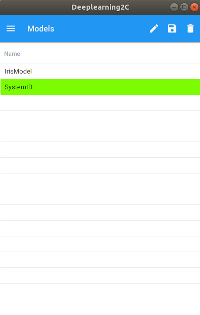
First I create my model.
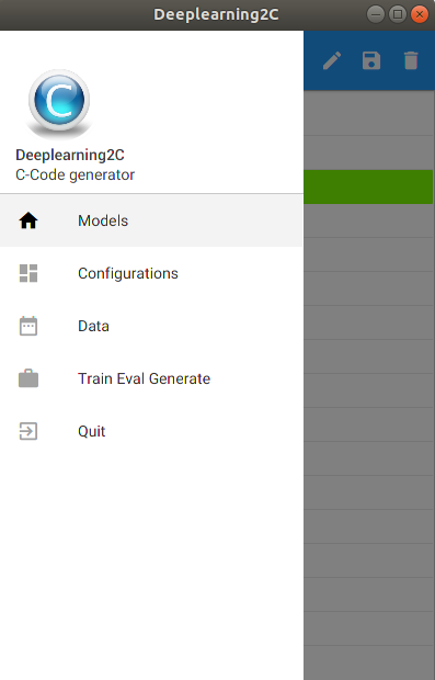
Then I go to menu.
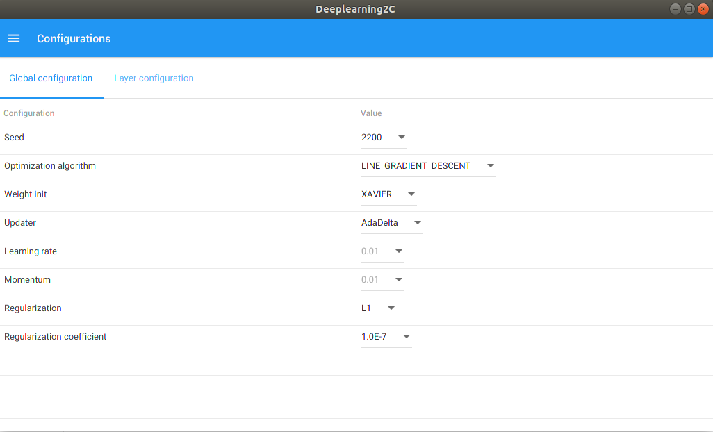
I change my global configuration.
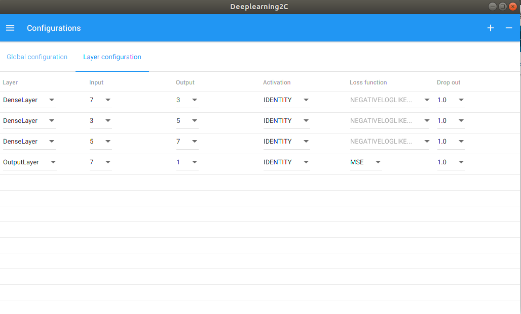
I change my layer configuration.
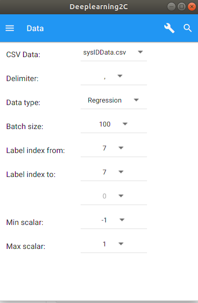
Then I insert the training data. Notice that 50% of that data is evaluation data.
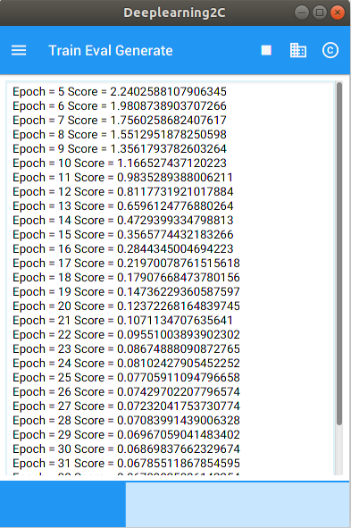
Now I train my model. Notice that I have a progress bar too.
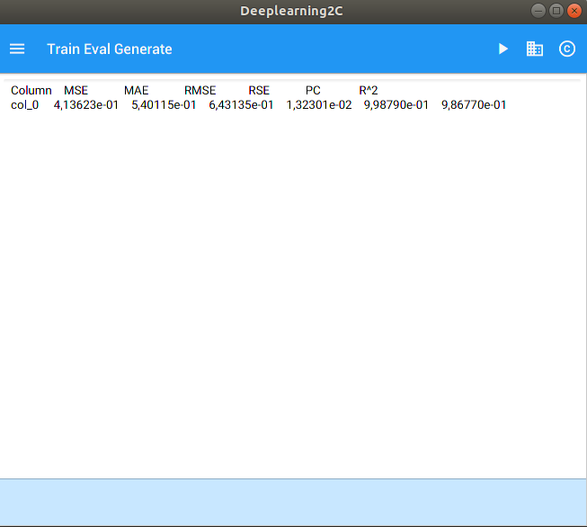
Now I evaluate my model.
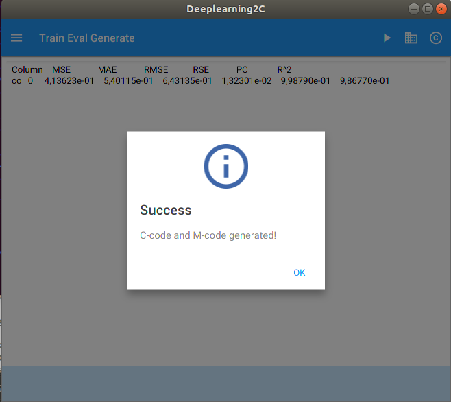
And at last I generate C-code and M-code.
This is how a setup looks like in C-code
/*
 ============================================================================
 Name        : IrisModelC.c
 Author      : Daniel Mårtensson
 Version     :
 Copyright   : MIT
 Description : Classification example
 ============================================================================
 */

#include <stdio.h>
#include <stdlib.h>
#include "IrisModel.h"

/*
 * This example has been trained with irisData.csv
 */
int main() {
	// Input
	float input[3][4] = {{4.4,3.0,1.3,0.2}, // Expected output: [1 0 0]
			     {6.5,2.8,4.6,1.5}, // Expected output: [0 1 0]
			     {6.7,3.0,5.2,2.3}}; // Expected output: [0 0 1]

	// Compute output
	float output[3] = {0,0,0};
	for(int i = 0; i < 3; i++){
		IrisModel(input[i], output);

		// Print result
		for(int j = 0; j < 3; j++){
			printf("Output %i = %f\n", j, output[j]);
		}
		printf("\n");
	}

	/*
	 * Result:
	 *  Output 0 = 0.999826
		Output 1 = 0.000173
		Output 2 = 0.000001

		Output 0 = 0.000038
		Output 1 = 0.999506
		Output 2 = 0.000456

		Output 0 = 0.000012
		Output 1 = 0.000806
		Output 2 = 0.999182
	 */

	return EXIT_SUCCESS;
}

/*
 * In MATLAB/GNU Octave it will look like this from the M-files folder
 *
 * >> IrisModel([4.4,3.0,1.3,0.2])
	ans =

	   9.9983e-01
	   1.7323e-04
	   1.0835e-06

	>> IrisModel([6.5,2.8,4.6,1.5])
	ans =

	   3.8034e-05
	   9.9951e-01
	   4.5604e-04

	>> IrisModel([6.7,3.0,5.2,2.3])
	ans =

	   1.1771e-05
	   8.0585e-04
	   9.9918e-01

	>>
 *
 */
This is how a C-code generation example looks like for this model.
/*
 * Model: IrisModel
 *
 *
 *  Created on: 2019-11-09 14:58:58
 *  	Generated by: Deeplearning2C
 *     		Author: Daniel Mårtensson
 */

#include "IrisModel.h"
#include "BLAS/f2c.h"
#include "BLAS/functions.h"

void IrisModel(float* input, float* output){

	integer m = 0; // Real row dimension of non-transpose A
	integer n = 0; // Real column dimension of non-transpose A
	real alpha = 1; // Always 1
	real beta = 1; // Always 1
	integer incx = 1; // Always 1
	integer incy = 1; // Always 1
	char trans = 'N'; // We have transpose matrix A'

	/*
	 * We are using BLAS subroutine sgemv for solving y = alpha*A*x + beta*y
	 * The BLAS subroutine is the same routine that is used in EmbeddedLapack
	 * Solve the equations like:
	 * b0 = act(W0*input + b0)
	 * b1 = act(W1*b0 + b1)
	 * b2 = act(W2*b1 + b2)
	 * b3 = act(W3*b2 + b3)
	 * b4 = act(W4*b3 + b4)
	 * ....
	 * ....
	 * output = act(Wi*b(i-1) + bi)
	 */

	real b0[1*3]={   -0.6087,    0.4616, 2.5645e-5};
	real W0[4*3]={   -0.8625,   -0.3397,   -0.4687,
			  0.2872,    0.8155,   -0.9267,
			  1.0887,    0.0980,   -0.4534,
			  0.3455,   -1.0067,   -0.1949};
	m = 3;
	n = 4;
	sgemv_(&trans, &m, &n, &alpha, W0, &m, input, &incx, &beta, b0, &incy); // Layer - first - index 0
	activation(b0, m, "TANH");

	real b1[1*5]={    0.2643,    0.3509,   -0.2505,    0.8730,    0.0396};
	real W1[3*5]={   -1.1832,    0.4539,    1.0578,   -1.1785,   -0.9066,
			  0.7488,   -1.0097,   -1.3093,    0.8479,    1.2361,
			  0.2831,   -0.8899,    0.1930,   -0.8783,    0.1381};
	m = 5;
	n = 3;
	sgemv_(&trans, &m, &n, &alpha, W1, &m, b0, &incx, &beta, b1, &incy); // Layer - middle - index 1
	activation(b1, m, "RELU");

	real b2[1*7]={    0.0912,    0.0025,   -0.1656,    0.0260,    0.3964,    0.0171,    0.0286};
	real W2[5*7]={   -0.7311,   -0.6416,    0.2090,   -0.1302,   -0.1392,    0.9976,   -0.3457,
			  0.5444,    0.6307,    0.6810,   -0.6130,    0.9825,   -0.9786,    0.5479,
			  1.4267,    0.5012,    0.5435,   -0.3866,   -0.4932,   -0.4949,    0.2377,
			 -0.7485,   -1.1880,   -0.9329,   -0.8541,    1.2560,    0.8988,   -1.0148,
			 -0.1380,   -0.2079,    0.6905,    0.0116,   -1.1755,    1.1405,    0.2818};
	m = 7;
	n = 5;
	sgemv_(&trans, &m, &n, &alpha, W2, &m, b1, &incx, &beta, b2, &incy); // Layer - middle - index 2
	activation(b2, m, "RELU");

	real b3[1*3]={   -0.3134,    0.4090,   -0.3947};
	real W3[7*3]={   -0.1978,    0.0382,    1.3856,
			  0.0070,   -0.7251,    0.7150,
			  0.1413,   -0.2986,    0.8372,
			  0.6356,   -0.2417,   -0.2545,
			 -0.9164,    1.7475,   -0.4681,
			  1.2910,   -0.9558,   -0.7706,
			  0.1475,   -0.5468,    1.7383};
	m = 3;
	n = 7;
	sgemv_(&trans, &m, &n, &alpha, W3, &m, b2, &incx, &beta, b3, &incy); // Layer - last - index 3
	activation(b3, m, "SOFTMAX");
	memcpy(output, b3, m*sizeof(float));

}
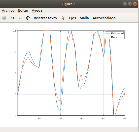
I also tried system identification.
%Model
sys = ss(0, [0 1; -1 -5], [0; 2], [1 0]);

% Signals
u1 = linspace(5,5, 100);
u2 = linspace(3,3, 100);
u3 = linspace(10,10, 100);
u4 = linspace(-4, -1, 100);
u5 = linspace(8, 9, 100);
u6 = 5*sin(linspace(0, 10, 100));
u7 = linspace(1, 10, 100);
u8 = linspace(10, 1, 100);
u9 = linspace(20, -20, 100);
u10 = linspace(0, 1, 100);
u = [u1 u2 u3 u4 u5 u6 u7 u8 u9 u10];

% Time
t = linspace(0, 100, length(u));

% Simulation with limits -5 and 15 on position and Inf on speed
y = satlsim(sys, u, t, [0;0], [-5 15; -Inf Inf]);

% Generate CSV file. Here we take adventage of transfer function estimation idea!
np = 5; % Number of poles
nz = 2; % Number of zeros

% check which one is largest
kn = length(u); % or length(y)

% Create b vector - all the y[k]
b = y(1:kn)';

% Create A1 matrix
A1 = zeros(kn, np);

% Fill A1 matrix - The y values
for i = 1:kn
  for j = 1:np

    if i-j <= 0
      A1(i,j) = 0;
    else
      A1(i,j) = -y(i-j);
    end

  end
end

% Create A2 matrix
A2 = zeros(kn, nz);

% Fill A2 matrix - The u values
for i = 1:kn
  for j = 1:nz

    if i-j <= 0
      A2(i,j) = 0;
    else
      A2(i,j) = u(i-j);
    end

  end
end

% Merge A1 and A2 into A
A = [A1 A2 b]; % This is ODE -y(t-1), -y(t-2), -y(t-3), -y(t-4), -y(t-5), u(t), u(t-1), y(t)
csvwrite('sysIDData.csv', A);

% Now we have trained our model and now we are doing a simulation
Y = zeros(1, np);
U = zeros(1, nz);
alpha = 2; % Reference scalar

for i = 1:length(u)
  % Insert signal u
  U = [u(i)*alpha U];
  U(end) = [];

  % Run model
  output = SystemID([Y U]);

  % Saturation
  if(output > 15)
    output = 15;
  elseif(output < -5)
    output = -5;
  end
  y(i) = output;

  % Insert output to Y
  Y = [-output Y]; % Important with negative output due to the ODE above
  Y(end) = [];

end

% Plot now the identified model
figure(2);
plot(t, y);
And here is the result. Remember that even if I have used a linear model, I still implemented limits = nonlinearities.
The M-file looks like this:
 %
 % Model: SystemID
 %
 %
 %  Created on: 2019-11-09 16:40:27
 %  	Generated by: Deeplearning2C
 %     		Author: Daniel Mårtensson
 %

function [output] = SystemID(input)

	 %
	 % We are solving y = A*x + y
	 % Solve the equations like:
	 % b0 = act(W0*input + b0)
	 % b1 = act(W1*b0 + b1)
	 % b2 = act(W2*b1 + b2)
	 % b3 = act(W3*b2 + b3)
	 % b4 = act(W4*b3 + b4)
	 % ....
	 % ....
	 % output = act(Wi*b(i-1) + bi)
	 %

	 b0=[   -0.1120,   -0.0402,    0.0032];
	 W0=[   -0.4450,    0.8477,   -0.2015,
		-0.1879,   -0.0192,   -0.8595,
		 0.3868,   -0.4800,   -0.3430,
		 0.1157,    0.3368,    0.2539,
		 0.1334,    0.0973,    0.4526,
		-0.1038,   -0.0941,    0.1836,
		-0.2202,   -0.0552,    0.7346];
	 b0 = act(W0'*input' + b0','IDENTITY'); % Layer - first - index 0
	 b1=[    0.0102,    0.0316,    0.0915,   -0.0355,   -0.0222];
	 W1=[    1.2714,    0.6818,   -0.3331,   -0.1709,   -0.4642,
		-0.2216,   -1.0645,    0.3952,    0.3615,    0.0884,
		-0.7550,    0.4536,   -0.0688,   -0.5332,   -0.5289];
	 b1 = act(W1'*b0 + b1','IDENTITY'); % Layer - middle - index 1
	 b2=[   -0.0227,   -0.0226,    0.0232,   -0.0238,   -0.0266,   -0.0021,    0.0443];
	 W2=[    0.0281,   -0.0413,    0.5902,   -0.0024,    0.0744,   -0.5026,   -0.4177,
		-0.0679,   -0.2938,   -0.1893,   -0.3184,   -0.3986,   -0.1307,    0.3192,
		 0.2063,    0.1591,   -0.0780,   -0.5964,   -0.1422,    0.0107,    0.2338,
		 0.1595,    0.2026,   -0.1367,   -0.3870,   -0.4170,    0.1332,    0.1796,
		 0.3216,    0.1110,   -0.5306,   -0.1794,   -0.6428,    0.3067,    0.3833];
	 b2 = act(W2'*b1 + b2','IDENTITY'); % Layer - middle - index 2
	 b3=[      0.0222];
	 W3=[     -0.6130,
		  -0.7850,
		   0.2164,
		  -0.1898,
		  -0.0856,
		  -0.5568,
		   0.0538];
	output = act(W3'*b2 + b3','IDENTITY'); % Layer - last - index 3
end
You need to have OpenJDK 8 and OpenJFX 8 installed. If you are a linux user, you can follow step 1 and 2.
- Install OpenJDK 8
sudo apt-get install openjdk-8-jdk
- Install OpenJFX 8
Open sources.list file

cd /etc/apt
sudo nano sources.list

Paste this into the file and save and close

deb http://de.archive.ubuntu.com/ubuntu/ bionic universe

Run these code inside the terminal

sudo apt-get update
sudo apt install openjfx=8u161-b12-1ubuntu2 libopenjfx-java=8u161-b12-1ubuntu2 libopenjfx-jni=8u161-b12-1ubuntu2 openjfx-source=8u161-b12-1ubuntu2
sudo apt-mark hold libopenjfx-java libopenjfx-jni openjfx openjfx-source
- Download the project and go to the project folder and run the command
./gradlew run
For Linux/Mac or
gradlew run
For Windows
I have been using Eclipse IDE.
- Install Eclipse 2018-09 (4.9.0) R (Because Eclipse 2018-09 will only work with Gluon Plugin 2.6.0)
https://www.eclipse.org/downloads/packages/release/2018-09/r
- Install Gluon Plugin 2.6.0 inside Eclipse
Help -> Eclipse Marketplace -> Gluon 2.6.0
First of all. The installation file is over 372 megabytes for Android. That's huge, but anyway it's still possible to install. Right now, I have excluded the most large dependencies which I don't use. Look in the build.gradle file.
-
See the getting started guide for using GluonHQ JavaFX for mobile development. It's a very easy and excellent done graphical manual. It describes how to set up the Android SDK etc. https://docs.gluonhq.com/getting-started/#introduction
-
Troubleshooting for Android can be done this way, if you got some issues with the application on the phone, but not on desktop. See selected answer https://stackoverflow.com/questions/42253794/androidinstall-task-causes-a-no-connected-devices-error
- Upgrade the C-code and M-code generator for LSTM networks.
I have always like clean god written code and pedagogy explanations. So I'm going to give you an introduction what every file do. I like to keep files as short as possible. Around 250-300 lines per each java file is a suitable java file.
- DrawerManager.java -> Handles the menu slide to the left
- Main.java -> Handles the import of new JavaFX pages
- DL4JData.java -> Handles everything that has to do with CSV handling for DL4J
- DL4JModel.java -> Handles everything that has to do with the model (save, load, generate etc.)
- DL4JSerializableConfiguration.java -> Handles saving and loading layers and global config to .ser files
- DL4JThread.java -> Handles training and using the text area and progress bar inside the TrainEvalGeneratePresenter.java file
- Dialogs.java -> Handles everything that has to do with pop-up dialogs
- FileHandler.java -> Handles file system, write files, read files and create files
- SimpleDependencyInjection.java -> Create a static object of DL4JModel.java so we can have access to DL4JModel everywhere
- ConfigurationsPresenter.java -> Handles GUI view for configuration
- DataPresenter.java -> Handles the GUI view for CSV import
- ModelsPresenter.java -> Handles the GUI view for model creation and delete/save
- TrainEvalGeneratePresenter.java -> Handles the GUI view for train, eval and generate C-code
Every file inside se.danielmartensson.views package that contains the word "View" inside its name is only for importing the GUI inside Main.java file. These files never changes.
- Tutorials -> Add seed, regularization coefficient, learning rate, momentum
- Tutorials -> Add new updater
- Tutorials -> Add new layer
- Tutorials -> Add inputs and outputs
- Tutorials -> Add new functionality to layers
