- mplfinance requires matplotlib and pandas
Start with a Pandas DataFrame containing OHLC data. For example,
import pandas as pd
daily = pd.read_csv('examples/data/SP500_NOV2019_Hist.csv',index_col=0,parse_dates=True)
daily.index.name = 'Date'
daily.shape
daily.head(3)
daily.tail(3)
(20, 5)
| Open | High | Low | Close | Volume | |
|---|---|---|---|---|---|
| Date | |||||
| 2019-11-01 | 3050.72 | 3066.95 | 3050.72 | 3066.91 | 510301237 |
| 2019-11-04 | 3078.96 | 3085.20 | 3074.87 | 3078.27 | 524848878 |
| 2019-11-05 | 3080.80 | 3083.95 | 3072.15 | 3074.62 | 585634570 |
...
| Open | High | Low | Close | Volume | |
|---|---|---|---|---|---|
| Date | |||||
| 2019-11-26 | 3134.85 | 3142.69 | 3131.00 | 3140.52 | 986041660 |
| 2019-11-27 | 3145.49 | 3154.26 | 3143.41 | 3153.63 | 421853938 |
| 2019-11-29 | 3147.18 | 3150.30 | 3139.34 | 3140.98 | 286602291 |
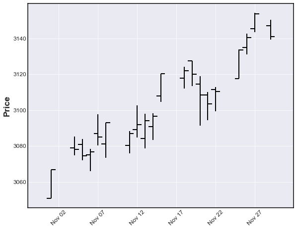
After importing mplfinance, plotting OHLC data is as simple as calling mpf.plot() on the dataframe
import mplfinance as mpf
mpf.plot(daily)
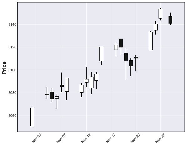
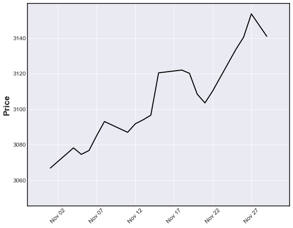
The default plot type, as you can see above, is 'ohlc'. Other plot types can be specified with the keyword argument type, for example, type='candle' or type='line'
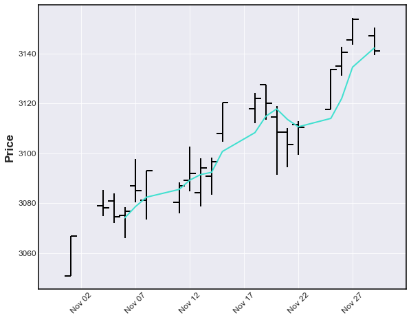
mpf.plot(daily,type='candle')mpf.plot(daily,type='line')We can also plot moving averages with the mav keyword
- use a scaler for a single moving average
- use a tuple or list of integers for multiple moving averages
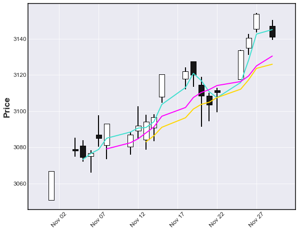
mpf.plot(daily,type='ohlc',mav=4)mpf.plot(daily,type='candle',mav=(3,6,9))We can also display Volume
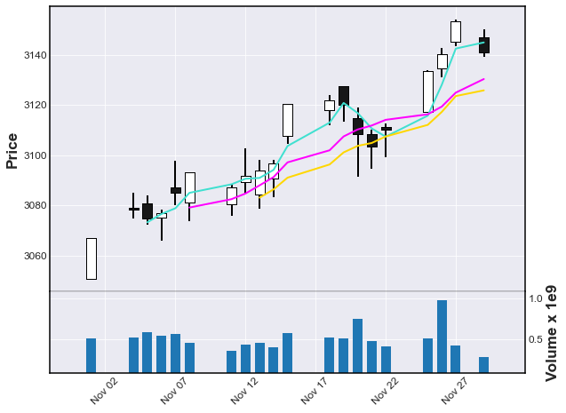
mpf.plot(daily,type='candle',mav=(3,6,9),volume=True)Notice, in the above chart, there are gaps along the x-coordinate corresponding to days on which there was no trading.
- Many people like to see these gaps so that they can tell, with a quick glance, where the weekends and holidays fall.
- For example, in the above chart you can see a gap at Thursday, November 28th for the U.S. Thanksgiving holiday.
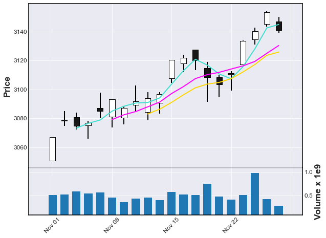
- Gaps along the x-axis can be eliminated with the
no_xgapskeyword
mpf.plot(daily,type='candle',mav=(3,6,9),volume=True,no_xgaps=True)We can also plot intraday data:
intraday = pd.read_csv('examples/data/SP500_NOV2019_IDay.csv',index_col=0,parse_dates=True)
intraday = intraday.drop('Volume',axis=1) # Volume is zero anyway for this intraday data set
intraday.index.name = 'Date'
intraday.shape
intraday.head(3)
intraday.tail(3)
(1563, 4)
| Open | Close | High | Low | |
|---|---|---|---|---|
| Date | ||||
| 2019-11-05 09:30:00 | 3080.80 | 3080.49 | 3081.47 | 3080.30 |
| 2019-11-05 09:31:00 | 3080.33 | 3079.36 | 3080.33 | 3079.15 |
| 2019-11-05 09:32:00 | 3079.43 | 3079.68 | 3080.46 | 3079.43 |
...
| Open | Close | High | Low | |
|---|---|---|---|---|
| Date | ||||
| 2019-11-08 15:57:00 | 3090.73 | 3090.70 | 3091.02 | 3090.52 |
| 2019-11-08 15:58:00 | 3090.73 | 3091.04 | 3091.13 | 3090.58 |
| 2019-11-08 15:59:00 | 3091.16 | 3092.91 | 3092.91 | 3090.96 |
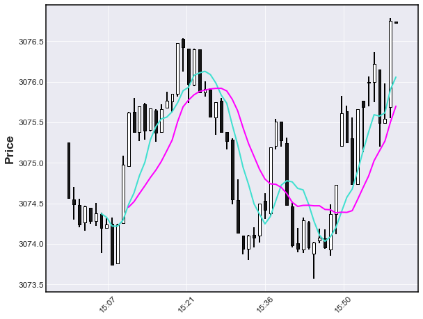
The above dataframe contains Open,High,Low,Close data at 1 minute intervervals for the S&P 500 stock index for November 5, 6, 7 and 8, 2019. Let's look at the last hour of trading on November 6th, with a 7 minute and 12 minute moving average.
iday = intraday.loc['2019-11-06 15:00':'2019-11-06 16:00',:]
mpf.plot(iday,type='candle',mav=(7,12))
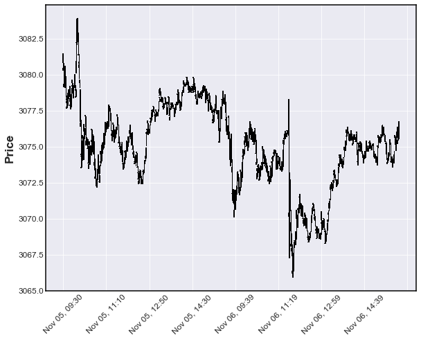
The "time-interpretation" of the mav integers depends on the frequency of the data, because the mav integers are number of data points used in the Moving Average. Notice above that for intraday data the x-axis automatically displays TIME instead of date. Below we see that if the intraday data spans two (or more) trading days then two things happen:
- The x-axis displays BOTH TIME and DATE
no-xgapsdefaults toTrueFOR INTRADAY DATA INVOLVING TWO OR MORE TRADING DAYS
iday = intraday.loc['2019-11-05':'2019-11-06',:]
mpf.plot(iday,type='candle')
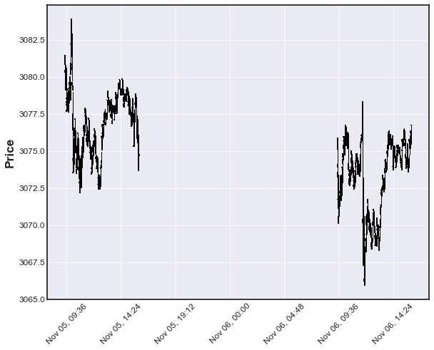
In the plot below, we see what would happen if no_xgaps did NOT default to True for intraday data involving two or more days.
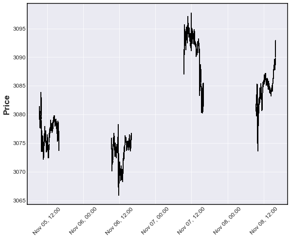
mpf.plot(iday,type='candle',no_xgaps=False)Below: 4 days of intraday data with no_xgaps=False
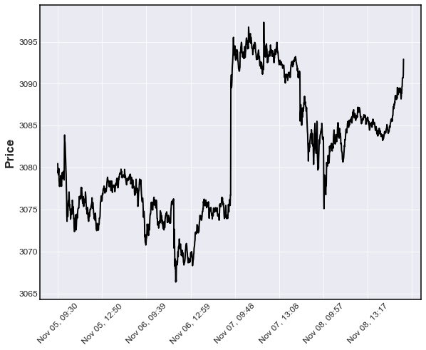
mpf.plot(intraday,type='ohlc',no_xgaps=False) # 4 day of intraday with no_xgaps=FalseBelow: 4 days of intraday data with no_xgaps defaulted to True for intraday data spanning more than one day.
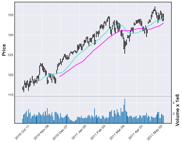
mpf.plot(intraday,type='line') # intraday spanning more than one day defaults to no_xgaps=TrueBelow: Daily data spanning more than a year automatically adds the YEAR to the DATE format
df = pd.read_csv('examples/data/yahoofinance-SPY-20080101-20180101.csv',index_col=0,parse_dates=True)
df.shape
df.head(3)
df.tail(3)
(2519, 6)
| Open | High | Low | Close | Adj Close | Volume | |
|---|---|---|---|---|---|---|
| Date | ||||||
| 2007-12-31 | 147.100006 | 147.610001 | 146.059998 | 146.210007 | 118.624741 | 108126800 |
| 2008-01-02 | 146.529999 | 146.990005 | 143.880005 | 144.929993 | 117.586205 | 204935600 |
| 2008-01-03 | 144.910004 | 145.490005 | 144.070007 | 144.860001 | 117.529449 | 125133300 |
...
| Open | High | Low | Close | Adj Close | Volume | |
|---|---|---|---|---|---|---|
| Date | ||||||
| 2017-12-27 | 267.380005 | 267.730011 | 267.010010 | 267.320007 | 267.320007 | 57751000 |
| 2017-12-28 | 267.890015 | 267.920013 | 267.450012 | 267.869995 | 267.869995 | 45116100 |
| 2017-12-29 | 268.529999 | 268.549988 | 266.640015 | 266.859985 | 266.859985 | 96007400 |
mpf.plot(df[700:850],type='bars',volume=True,no_xgaps=True,mav=(20,40))For more examples of using mplfinance, please see the jupyter notebooks in the examples directory.
- customize appearance of plot (colors, date format, etc)
- show trading signals on plot
- technical studies, such as:
- Trading Envelope, Bollinger Bands
- MACD
- custom studies and/or additional data on plot
- Ability to plot specified additional columns from DataFrame either within the main ohlc plot, or only the lower axis where volume may be displayed.
- save plot to file
My name is Daniel Goldfarb. In November 2019, I became the maintainer of matplotlib/mpl-finance. That module is being deprecated in favor of the current matplotlib/mplfinance. The old mpl-finance consisted of code extracted from the deprecated matplotlib.finance module along with a few examples of usage. It has been mostly un-maintained for the past three years.
It is my intention to archive the matplotlib/mpl-finance repository soon, and direct everyone to matplotlib/mplfinance. The main reason for the rename is to avoid confusion with the hyphen and the underscore: As it was, mpl-finance was installed with the hyphen, but imported with an underscore mpl_finance. Going forward it will be a simple matter of both installing and importing mplfinance.
At present (Dec 2019) this repository, matplotlib/mplfinance, contains an initial 'alpha', version of the new API for people to play with and provide feedback or pull requests for enhancements.
My own take on the old mpl-finance API is that the methods were too low-level, and too cumbersome to use. The new API in this current package automatically does the extra matplotlib work that the caller previously had to do "manually, on their own" with the old API.
The conventional way to import the new API is as follows:
import mplfinance as mpfThe most common usage is to then call mpf.plot(data) where data is a Pandas DataFrame object containing Open, High, Low and Close data, with a Pandas DatetimeIndex.
I am very interested to hear from you regarding how you were using the old mpl-finance (if you were), what you think of the new mplfinance, plus any suggestions you may have for improvement. You can reach me at dgoldfarb.github@gmail.com
With this new mplfinance package installed, in addition to the new API, users can still access the old API (at least for the next several months) by changing their import statments
from:
from mpl_finance import <method>to:
from mplfinance.original_flavor import <method>where <method> indicates the method you want to import, for example:
from mplfinance.original_flavor import candlestick_ohlc