4. Fitting
Spinmob provides a nonlinear least-squares fitter based on the lmfit package. It is capable of fitting arbitrary curves to an arbitrary number of data sets simultaneously while (optionally) providing an interactive visualization of the data, functions, and residuals. It also allows you to non-destructively pre-process the data (trim, coarsen), fix parameters, constrain parameters, and more.
The primary goal of this object, however, is to lower the barrier between your data and a research-grade fitting engine.
In []: import spinmob as sFirst let's make a fitter object:
In []: f = s.data.fitter()Let's inspect the object by typing its name:
In []: my_fitter
Out[]:

FITTER SETTINGS
  autoplot        True
  coarsen         [1]
  first_figure    0
  fpoints         [1000]
  plot_all_data   [False]
  plot_bg         [True]
  plot_errors     [True]
  plot_fit        [True]
  plot_guess      [True]
  plot_guess_zoom [False]
  scale_eydata    [1.0]
  silent          False
  style_bg        [{'marker': '', 'color': 'k', 'ls': '-'}]
  style_data      [{'marker': 'o', 'color': 'b', 'ls': '', 'mec': 'b'}]
  style_fit       [{'marker': '', 'color': 'r', 'ls': '-'}]
  style_guess     [{'marker': '', 'color': '0.25', 'ls': '-'}]
  subtract_bg     [False]
  xlabel          [None]
  xmax            [None]
  xmin            [None]
  xscale          ['linear']
  ylabel          [None]
  ymax            [None]
  ymin            [None]
  yscale          ['linear']

INPUT PARAMETERS

NO FIT RESULTS
Look at all those settings! You can change any of them using the set() function, e.g., f.set(ymin=32, plot_guess=False) and retrieve their values with dictionary-like indexing, e.g., f['ymin']. These settings will affect how the data is processed, and how it is visualized. As a shortcut, calling f() is identical to f.set(), so the same could be achieved with f(ymin=32, plot_guess=False).
Let's now specify a function we will use to fit some data:
In []: f.set_functions('a*x+cos(b*x)+c', 'a,b=2,c')Here, the first argument is the function (in this case a string), the second is a comma-delimited list of fit parameters (also a string), with optional guess values. Function strings are exposed to all of numpy (e.g. cos and sqrt), and you can include your own dictionary of globals via set_functions()'s g argument (or simply as additional keyword arguments), i.e.,
In []: f.set_functions('a*x + cos(b*x)   + c', 'a,b=2,c')
In []: f.set_functions('a*x + pants(b*x) + c', 'a,b=2,c', pants=numpy.cos)
In []: f.set_functions('a*x + pants(b*x) + c', 'a,b=2,c', g={'pants':numpy.cos})
are all equivalent (provided you have imported numpy!). This is especially useful if you want to define your own arbitrarily complicated function with, e.g., for loops or something fancy-pants inside.
You can always set guess values later using set() as above, e.g., f.set(c=12.2) or f(c=12.2) as a shortcut. For the first argument, you can specify a single function, as shown above, or list of functions for simultaneously fitting multiple data sets. You can furthermore specify constant parameters and/or background functions of the same parameters (see below or help(f.set_functions)).
INPUT PARAMETERS
  a = 1, vary=1 min=-INF max=INF expr=None
  b = 2, vary=1 min=-INF max=INF expr=None
  c = 1, vary=1 min=-INF max=INF expr=None

NO FIT RESULTS
The fitter engine is now primed with three parameters, with initial guess values a=1, b=2, and c=1 (the default guess is always 1).
All settings, constants, and parameter guesses can be set with either the f.set() or f() function. For example, f(a=3.2, xmin=1, xmax=4).
In []: f.set_data(xdata=[1,2,3,4,5], ydata=[1,2,1,4,3], eydata=0.7)All three arguments can be numpy arrays (Perhaps databox columns? See 2. Data Handling) or lists of numpy arrays (with length matching the number of functions!). Using the default settings, the command above should pop up a plot of the data (blue) and guess (gray):

The way (or whether) these things are plotted can be changed using f.set() as described above. Note for multiple data sets, if you only supply one xdata set, it will assume the same xdata for each ydata set.
In []: f.fit()This will perform the least-squares minimization, updating the plots and residuals:
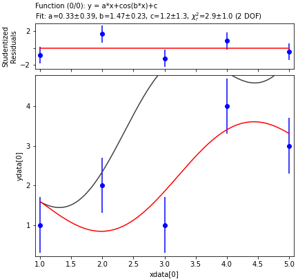
You can see the results of the fit on the plot or by again inspecting the f object as we did in step 1. The output of scipy.optimize.leastsq() is stored in f.results. It is a list, the first element is an array of fit parameters, and the second element is the covariance matrix. See the leastsq documentation for additional info.
Note that if you do not specify the y error bars (eydata) the fitter will make a completely arbitrary guess based on the max and min values of the supplied data. As a result, the reduced chi^2 will be meaningless, the parameter errors / correlations will be totally wrong, and your eyes will eventually cease to smile when your mouth does. You should always estimate and justify your errors, undergrads, because I am grading your reports. However, if you are not my student and you just want a dirty estimate of the error in the fit parameters, you can cheat a bit using f.autoscale_eydata_and_fit() a few times until your reduced chi^2 is 1. Use at your own risk: this basically amounts to estimating the error by sampling the data (which contains the science you are trying to fit!) itself, and assumes that your curve perfectly describes the data and that the errors are totally random, Gaussian, and uncorrelated. Good luck explaining this on a final report, much less how all of your reduced chi^2 values happen to be exactly 1.
You can also specify "background functions" by setting the parameter bg just as you do for f. For example:
In []: f = s.data.fitter()
In []: f.set_functions(f='a/(1.0+(x-x0)**2/w**2) + b + c*x',
                       p='a=1, x0=1, w=1, b=0, c=0',
                       bg='b+c*x')
In []: f.set_data([1,2,3,4,5,6,7], [1,2,3.5,2,1,0,-1], 0.3).fit()
will produce this:

Notice both the guess and fit functions now display the specified background function, for reference. The background function is purely for visualization and has no effect on the fit. Specifying bg essentially amounts to specifying what part of the fit function is due to background.
If you like, you can specify that the background function be subtracted from the data prior to plotting by setting f(subtract_bg=False). The result is then:

Notice the fit background was subtracted from everything, including the guess (which is why the guess is skewed despite the guess c being 0). Prior to the fit, however, the guess background will be subtracted from everything.
Sometimes it is difficult to include the fit function model into a string. Instead of inputing a string to the fitter, you can also input an arbitrarily complicated function. For example, suppose we have the function:
def loud_cos(x, a, b, c):
    """
    Loud cosine with an offset, 'a*x*cos(b*x)+c'.
    """

    # Make some noise (or do crazy calculations)
    for n in range(10): print("Yay!")

    # Return some cosine
    return a * x * np.cos(b*x) + c
You can then set the f parameter of the fitter to this function directly:
f = s.data.fitter()
f.set_functions(f=loud_cos, p='a,b,c')
Note this technique requires that the function takes the "x" data as the first parameter, and the fit parameters as the rest, and that the user-specified parameter list match the order of the parameter list in the function. Alternatively (my preferred method), you can use a globally defined function within the usual function string, e.g.:
f = s.data.fitter()
f.set_functions(f='d+y(x,a,b,c)**2', p='d,b,c,a', y=loud_cos)
In this case, you must also specify what y means (the final argument) so the fitter knows what these objects actually are. Here I used y in the function string, and specified that y is loud_cos so the fitter will know what to do with y when it sees it. You can send as many special objects as you like using additional keyword arguments. (For older versions of spinmob, specify a "globals dictionar", as the keyword argument `g=dict(y=loud_cos)'.)
You can also specify multiple data sets and a function to fit each using the same set of parameters. You accomplish this by sending a list of functions and a list of data sets, for example:
f = s.data.fitter()
f.set_functions(['a*sin(x)+b', 'a+b*x+c**2'], p='a,b,c')
f.set_data([[1,2,3,4,5], [1,2,3,4,5]], [[1,3,1,4,1], [1,5,1,5,1]], 1.2)
In this case, a figure for each data set should pop up, and you can then proceed as normal. The default arguments for s.data.fitter() and f.set_data() have another an example of this.
These are some of the more commonly used functions when fitting (assumes your fitter object is called f).
-
f.set()orf()- allows you to change one or more parameters or settings -
f.ginput()- click the specified figure to get x,y values (great for guessing!) -
f.trim()- keeps only the currently visible data for fitting (use the zoom button on the graph!) -
f.untrim()- removes trim. -
f.zoom()- zooms out or in (trimming) -
f.fix()- fix one or more of the parameters -
s.tweaks.ubertidy()- auto-formats figure for Inkscape (use the save button on the graph and save in 'svg' format) -
f(a=11, b=2, plot_guess=False)- change some guess values and settings (disabling the guess plot) -
f(coarsen=3, subtract_bg=[True, False])- coarsen the data (by averaging every 4 data points) prior to fitting (```coarsen=0''' means "no coarsening"), and also subtract the background function from only the first data set.
Note when changing a setting, specifying a list allows you to change settings for each plot, and specifying just a value will change the setting for all plots.
Most of the settings are self-explanatory (just try them!), but my favorites are
- coarsen - how much to bin/average the data prior to fitting (0 means "no coarsening")
- xmin, xmax - x-range over which we should actually fit the data
Enjoy!
Up next: 5. Settings, Dialogs, Printing