- Identified the optimal sample size for the desired significance level and statistical power
- Generated a realistic data set using simulation techniques for study design
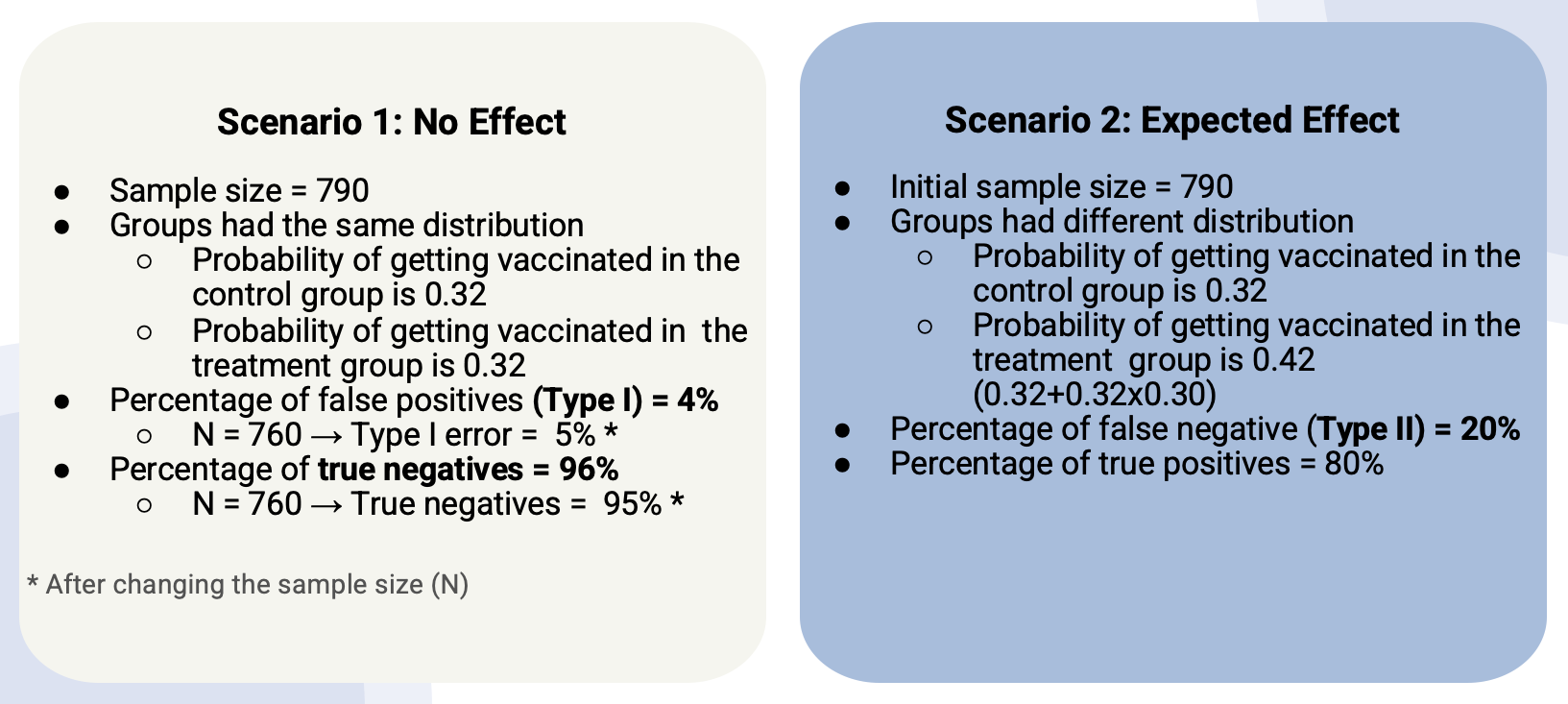
- Created two scenarios: one with the expected effect and another with no effect
- Analyzed the simulation data in both scenarios
- There is vast literature suggesting that incentive rewards motivate people to change health behaviors (Seal et al., 2003; Gong et al., 2018)
- A survey experiment by the U.C.L.A. suggests that approximately a third of the U.S. unvaccinated population reported they would be more likely to get the vaccine with a monetary incentive (New York Times, 2021)
- The literature also suggests that tailored interventions have the potential to improve health behavior (Krebs et al., 2010; McCurley et al., 2017)
Louisiana has the 4th lowest COVID-19 vaccine rate, with only 42% of the adult population with at least one vaccine dose
Research Question:
What effect do tailored incentives have on the COVID-19 vaccine rate?
Incentive Offer:
- Lottery entry with five winners selected at random, who will each receive 2 Saints football season tickets for the 2021 season
- 75% of New Orleans residents identify as Saints fans. Top 3 most passionate sports fans in America
Null Hypothesis: The proportion of participants who get at least one dose of the COVID-19 vaccine will be the same between the control group (defined as participants who were mailed a flyer without an incentive) and the treatment group (defined as the participants who were sent a flyer with an incentive)
Alternative Hypothesis: The proportion of participants who get at least one dose of the COVID-19 vaccine will not be the same between the control group (defined as participants who were mailed a flyer without an incentive) and the treatment group (defined as the participants who were sent a flyer with an incentive)
The Population of Interest: Gen Z & Millennials who live in New Orleans that have not yet been vaccinated
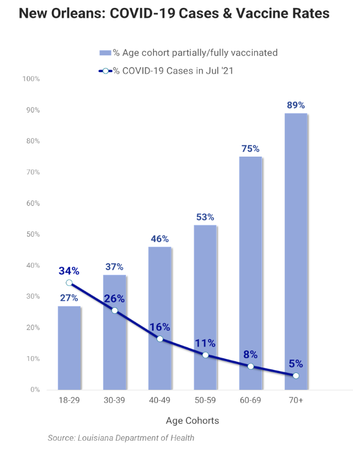
- New Orleans has been the hotspot in Louisiana, with 17% of the state's COVID-19 cases
- Only 32% of Gen Z & Millennials are partially vaccinated, compared to 64% of adults 40 years and older
Operational Procedures:
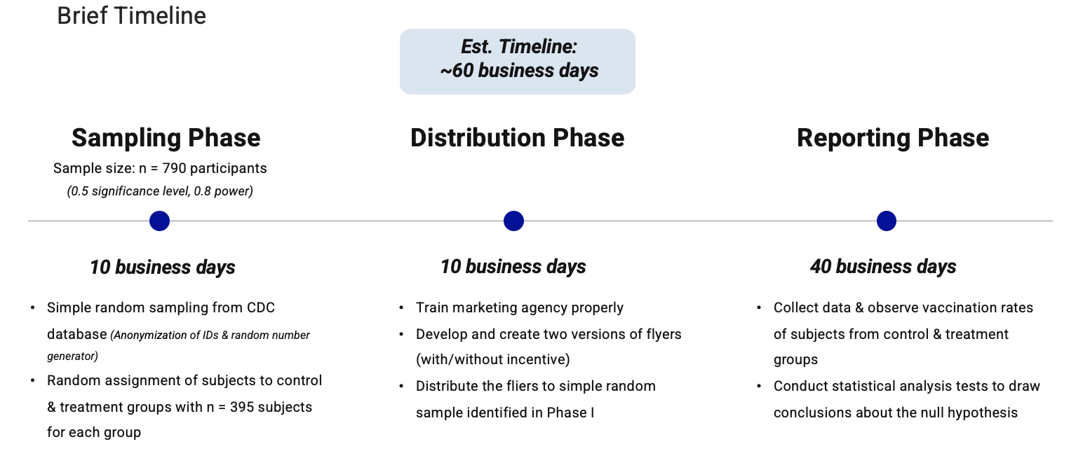
Statistical Plan:
Sample Size Estimation:
- Current vaccination rate = 32%
- Estimated treatment rate = 42%
- A recent study suggests that 34% of unvaccinated adults would be more likely to get vaccinated with a cash payment (New York Times, 2021)
- For the present simulation, we used 32% as the expected additional vaccination probability for the treatment group
- We used 32% instead of 34% to account for the difference between what participants said they will do vs. what they do
# p1 = control = no incentive
# p2 = treatment = with incentive

library(pwr)
power.prop.test(p1= .32, p2= (.32 + 0.32*0.30), sig.level = 0.05, power = .8)
library(data.table)
library(DT)
library(purrr)

n <- 790
set.seed(seed = 329)

bp.dat <- data.table(Group = sample(x = c("Treatment", "Control"), size = n, replace = T))

bp.dat[Group == "Treatment", VR := round(x = rbernoulli(n = .N, p=.32), digits = 1)]
bp.dat[Group == "Control", VR := round(x = rbernoulli(n = .N, p=.32), digits = 1)]

table(bp.dat)
           VR
Group         0   1
  Control   281 137
  Treatment 246 126
prop.test(table(bp.dat$Group, bp.dat$VR))
    2-sample test for equality of proportions with continuity correction

data:  table(bp.dat$Group, bp.dat$VR)
X-squared = 0.062809, df = 1, p-value = 0.8021
alternative hypothesis: two.sided
95 percent confidence interval:
 -0.05744408  0.07936104
sample estimates:
   prop 1    prop 2
0.6722488 0.6612903
analyze.experiment <- function(the.dat) {
  setDT(the.dat)

  the.test <- prop.test(table(the.dat$Group, the.dat$VR))

  the.effect <- the.test$estimate[1] - the.test$estimate[2]
  lower.bound <- the.test$conf.int[1]
  p <- the.test$p.value

  result <- data.table(effect = the.effect, lower_ci = lower.bound, p = p)

  return(result)
}

analyze.experiment(the.dat = bp.dat)
       effect    lower_ci         p
1: 0.01095848 -0.05744408 0.8021103
table(bp.dat)
           VR
Group         0   1
  Control   281 137
  Treatment 246 126
prop.test(table(bp.dat$Group, bp.dat$VR))
Scenario 1 Analysis
n <- 790
B <- 1000
RNGversion(vstr = 3.6)
set.seed(seed = 4172)

Experiment <- rep.int(x = 1:B, times = n)
Group <- sample(x = c("Treatment", "Control"), size = n*B, replace = T)

sim.dat <- data.table(Experiment, Group)
setorderv(x = sim.dat, cols = c("Experiment", "Group"), order = c(1,1))
sim.dat[Group == "Treatment", VR := round(x = rbernoulli(n = .N, p=.32), digits = 1)]
sim.dat[Group == "Control", VR := round(x = rbernoulli(n = .N, p=.32), digits = 1)]

dim(sim.dat)
[1] 790000 3
exp.results <- sim.dat[, analyze.experiment(the.dat = .SD),
                       keyby = "Experiment"]

DT::datatable(data = round(x = exp.results[1:100, ], digits = 3),
    rownames = F)
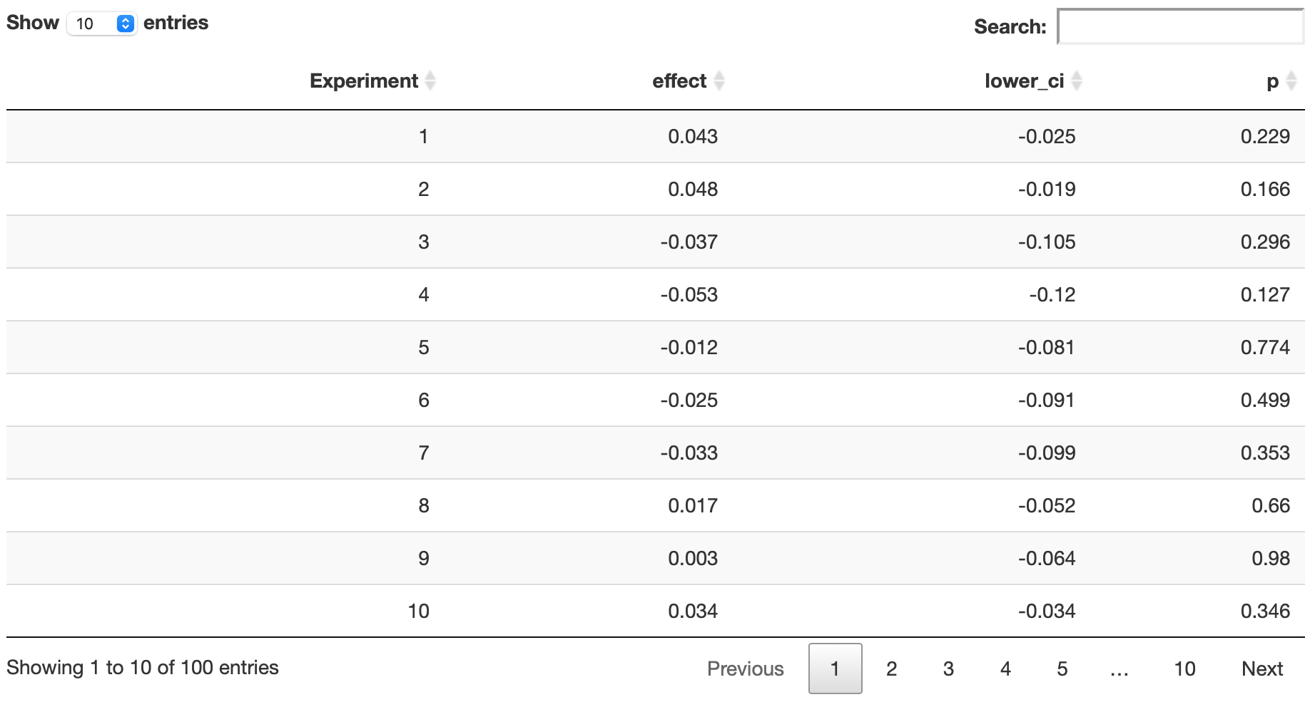
exp.results[, mean(p < 0.05)]
[1] 0.035
exp.results[, summary(effect)]
     Min.   1st Qu.    Median      Mean   3rd Qu.      Max.
-0.101412 -0.021927  0.001065  0.000511  0.023402  0.125469
exp.results[, summary(lower_ci)]
    Min.  1st Qu.   Median     Mean  3rd Qu.     Max.
-0.16727 -0.08955 -0.06528 -0.06695 -0.04394  0.05961
n <- 790
set.seed(seed = 329)

bp.dat <- data.table(Group = sample(x = c("Treatment", "Control"), size = n, replace = T))
bp.dat[Group == "Treatment", VR := round(x = rbernoulli(n = .N, p=.32 + 0.32*0.30), digits = 1)]
bp.dat[Group == "Control", VR := round(x = rbernoulli(n = .N, p=.32), digits = 1)]

table(bp.dat)
           VR
Group         0   1
  Control   281 137
  Treatment 207 165
prop.test(table(bp.dat$Group, bp.dat$VR))
    2-sample test for equality of proportions with continuity correction

data:  table(bp.dat$Group, bp.dat$VR)
X-squared = 10.692, df = 1, p-value = 0.001076
alternative hypothesis: two.sided
95 percent confidence interval:
 0.04562873 0.18596565
sample estimates:
   prop 1    prop 2
0.6722488 0.5564516
analyze.experiment <- function(the.dat) {
  setDT(the.dat)

  the.test <- prop.test(table(the.dat$Group, the.dat$VR))

  the.effect <- the.test$estimate[1] - the.test$estimate[2]
  lower.bound <- the.test$conf.int[1]
  p <- the.test$p.value

  result <- data.table(effect = the.effect, lower_ci = lower.bound, p = p)

  return(result)
}

analyze.experiment(the.dat = bp.dat)
      effect   lower_ci           p
1: 0.1157972 0.04562873 0.001076139
Scenario 1 Analysis
n <- 820
B <- 1000

RNGversion(vstr = 3.6)
set.seed(seed = 4172)

Experiment <- rep.int(x = 1:B, times = n)
Group <- sample(x = c("Treatment", "Control"), size = n*B, replace = T)

sim.dat <- data.table(Experiment, Group)
setorderv(x = sim.dat, cols = c("Experiment", "Group"), order = c(1,1))
sim.dat[Group == "Treatment", VR := round(x = rbernoulli(n = .N, p=.32 + 0.32*0.30), digits = 1)]
sim.dat[Group == "Control", VR := round(x = rbernoulli(n = .N, p=.32), digits = 1)]

dim(sim.dat)
[1] 820000 3
names(sim.dat)
[1] "Experiment" "Group" "VR"
exp.results <- sim.dat[, analyze.experiment(the.dat = .SD),
                       keyby = "Experiment"]


DT::datatable(data = round(x = exp.results[1:100, ], digits = 3),
    rownames = F)

exp.results[, mean(p < 0.05)]
[1] 0.801
exp.results[, summary(effect)]
    Min.  1st Qu.   Median     Mean  3rd Qu.     Max.
-0.03328  0.07413  0.09578  0.09614  0.11955  0.21595
exp.results[, summary(lower_ci)]
     Min.   1st Qu.    Median      Mean   3rd Qu.      Max.
-0.100707  0.006117  0.027686  0.028056  0.051713  0.148724
- Optinal sample size for this study is 790
- Probability of false positives (Type I) = 4%
- Probability of false negative (Type II) = 20%