Originally put together for a mini-workshop on 8 Nov. 2019 in Gothenburg, Sweden.
supersmartRis a series of R packages that form a phylogenetic pipeline.- The original SUPERSMART program uses a "divide-and-conquer" apprach to constructing large phylogenetic trees.
- It combines both a supermatrix (an assembly of multiple gene/clusters into a single matrix) and a supertree (merging multiple trees) approach.
supersmartRpackages are standalone packages with their own functions and uses BUT they can be combined to recreate the supersmart pipeline.

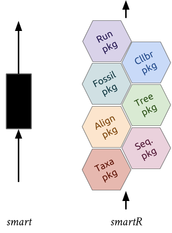
This workshop we will introduce the packages and provide code to run a simple pipeline to create a phylogenetic tree (a supertree of all Guinea-pig-like species).
- Introduction to
phylotaR - Introduction to
restez - Introduction to
outsider - Introduction to
gaius - Supertree pipeline
Target Duration ~1 hr
- Software
- R (> 3.5)
- RStudio
- Desktop Docker (Linux containers)
- Basic knowledge
- R
- Phylogenetics
(Windows users may struggle installing Docker Desktop, in which case Docker Toolbox will also work.)
Install dependant packages.
# remotes allows installation via GitHub
if (!'remotes' %in% installed.packages()) {
  install.packages('remotes')
}

library(remotes)
# install latest outsider
install_github("antonellilab/outsider.base")
install_github("antonellilab/outsider")
# install latest restez
install_github("hannesmuehleisen/MonetDBLite-R")
install_github("ropensci/restez")
# install latest phylotaR
install_github("ropensci/phylotaR")
# install latest gaius
install_github("antonellilab/gaius")
If you're computer is set-up correctly with the R packages and Docker, you should be able to run the below script without errors (don't worry about security warnings).
## Code
library(outsider)
#> ----------------
#> outsider v 0.1.0
#> ----------------
#> - Security notice: be sure of which modules you install
repo <- "dombennett/om..hello.world"
module_install(repo = repo, force = TRUE)
hello_world <- module_import(fname = "hello_world", repo = repo)
hello_world()

## Output
#> Hello world!
#> ------------
#> DISTRIB_ID=Ubuntu
#> DISTRIB_RELEASE=18.04
#> DISTRIB_CODENAME=bionic
#> DISTRIB_DESCRIPTION="Ubuntu 18.04.1 LTS"To run all the code in this workshop you will need to:
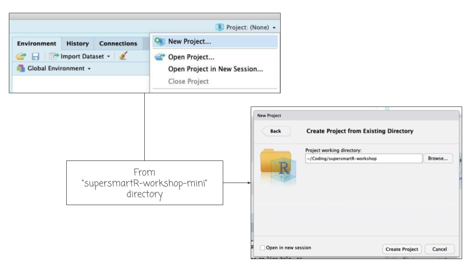
- Download the zipped folder of this GitHub repo, click here.
- Unzip this folder and place it in a convenient location on your computer (e.g. "my coding projects").
- Open RStudio and create a new project from this new folder.
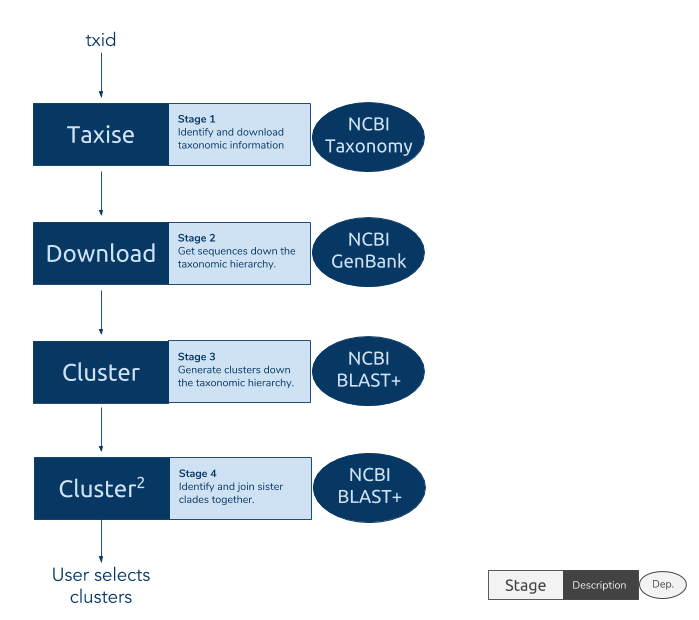
The phylotaR package downloads all sequences associated with a given taxonomic group and then runs all-vs-all BLAST to identify clusters of sequences suitable for phylogenetic analysis.
The process takes place across four stages:
- Taxise: identify taxonomic IDs
- Download: download sequences
- Cluster: run all-vs-all BLAST
- Cluser^2: run all-vs-all BLAST again
To run phylotaR, we need to set up a folder to host all downloaded files. Parameters for setting up the folder are provided to the setup function.
# NOT RUN
library(phylotaR)
# available parameters
print(parameters())
# e.g. mnsql = 200 - minimum sequence length
# pass the parameters to the setup() function
# essential parmeters are: wd, txid
wd <- file.path(tempdir(), 'testing_phylotaR')
if (dir.exists(wd)) {
  unlink(x = wd, recursive = TRUE, force = TRUE)
}
dir.create(wd)
setup(wd = wd, txid = '9504', outsider = TRUE, v = TRUE)
# to run the pipeline
# run(wd = wd)Read in the phylotaR results with read_phylota. But here we will use the pacakge example data, "Aotus".
library(phylotaR)
data(aotus)
# generate summary stats for each cluster
smmry_tbl <- summary(aotus)
# Important details
#  N_taxa     - number of taxonomic entities associated with sequences in cluster
#  N_seqs     - number of sequences in cluster
#  Med_sql    - median sequence length of sequences in cluster
#  MAD        - measure of the deviation in sequence length of a cluster
#  Definition - must common words in sequence definition lines
smmry_tbl[1:10, ]
#>    ID    Type               Seed Parent N_taxa N_seqs Med_sql       MAD
#> 1   0 subtree         AF129794.1   9504      5    204     267 0.7124669
#> 2   1 subtree           U52114.1   9504      5     63    1020 0.7604098
#> 3   2 subtree         DI178118.1   9504      2     52     267 0.8666904
#> 4   3 subtree         JQ932794.1   9504      4     43     568 0.6643121
#> 5   4 subtree           U36844.1   9504      9     41     549 0.8397112
#> 6   5 subtree KF014117.1/1..1263   9504      1     35    1281 0.7731248
#> 7   6 subtree         LC075891.1   9504      2     33     838 0.8026216
#> 8   7 subtree         JN161069.1   9504      1     30    1088 0.9985614
#> 9   8 subtree         JN161069.1  30591      1     30    1088 0.9985614
#> 10  9 subtree         AJ489745.1   9504     10     29    1140 1.0000000
#>                           Definition                      Feature
#> 1       aotus (0.07), partial (0.07) aovodrb (0.5), aonadrb (0.5)
#> 2         aotus (0.09), class (0.09)                     mhcf (1)
#> 3  antibody (0.05), construct (0.05)           jp (0.3), kr (0.2)
#> 4         aotus (0.2), genomic (0.2)                            -
#> 5    gene (0.1), mitochondrial (0.1)                     coii (1)
#> 6        allele (0.08), aotus (0.08) kir3ds3 (0.2), kir2ds5 (0.1)
#> 7             dna (0.1), aotus (0.1)                            -
#> 8          azarai (0.2), aotus (0.1)                            -
#> 9          azarai (0.2), aotus (0.1)                            -
#> 10     aotus (0.1), cytochrome (0.1) cytb (0.4), cytochrome (0.3)
# plot
p <- plot_phylota_treemap(phylota = aotus, cids = aotus@cids[1:10],
area = 'nsq', fill = 'ntx')
print(p)
# CODE

# PhyLoTa table has ...
# clusters
aotus@clstrs
# sequences
aotus@sqs
# taxonomy
aotus@txdct
# A cluster is a list of sequences
aotus@clstrs@clstrs[[1]]
str(aotus@clstrs@clstrs[[1]])
# A sequence is a series of letters and associated metadata
aotus@sqs@sqs[[1]]
str(aotus@sqs@sqs[[1]])
# A taxonomic record is an ID and associated metadata
txid <- aotus@txids[[1]]
# Information can be extracted from ...
# clusters
get_clstr_slot(phylota = aotus, cid = aotus@cids[1:10], slt_nm = 'nsqs')
# sequences
get_sq_slot(phylota = aotus, sid = aotus@sids[1:10], slt_nm = 'nncltds')
# tax. records
get_tx_slot(phylota = aotus, txid = aotus@txids[1:10], slt_nm = 'scnm')
# Other useful convenience functions
get_nsqs(phylota = aotus, cid = aotus@cids[1:10])
get_ntaxa(phylota = aotus, cid = aotus@cids[1:10], rnk = 'species')

# OUTPUT
#> Archive of cluster record(s)
#>  - [193] clusters
#> Archive of sequence record(s)
#>  - [1499] sequences
#>  - [13] unique txids
#>  - [548] median sequence length
#>  - [0] median ambiguous nucleotides
#> Taxonomic dictionary [21] recs, parent [id 9504]
#> Cluster Record [id 0]
#>  - [subtree] type
#>  - [AF129794.1] seed sequence
#>  - [204] sequences
#>  - [5] taxa
#> Formal class 'ClstrRec' [package "phylotaR"] with 8 slots
#>   ..@ id   : int 0
#>   ..@ sids : chr [1:204] "AF129792.1" "AF129793.1" "AF129794.1" "AF129795.1" ...
#>   ..@ nsqs : int 204
#>   ..@ txids: chr [1:204] "231953" "231953" "231953" "231953" ...
#>   ..@ ntx  : int 5
#>   ..@ typ  : chr "subtree"
#>   ..@ prnt : chr "9504"
#>   ..@ seed : chr "AF129794.1"
#> SeqRec [ID: FJ623078.1]Formal class 'SeqRec' [package "phylotaR"] with 16 slots
#>   ..@ id     : chr "FJ623078.1"
#>   ..@ nm     : chr ""
#>   ..@ accssn : chr "FJ623078"
#>   ..@ vrsn   : chr "FJ623078.1"
#>   ..@ url    : chr "https://www.ncbi.nlm.nih.gov/nuccore/FJ623078.1"
#>   ..@ txid   : chr "37293"
#>   ..@ orgnsm : chr "Aotus nancymaae"
#>   ..@ sq     : raw [1:1374] 61 74 67 67 ...
#>   ..@ dfln   : chr "Aotus nancymaae CD4 antigen (CD4) mRNA, complete cds"
#>   ..@ ml_typ : chr "mRNA"
#>   ..@ rec_typ: chr "whole"
#>   ..@ nncltds: int 1374
#>   ..@ nambgs : int 0
#>   ..@ pambgs : num 0
#>   ..@ gcr    : num 0.447
#>   ..@ age    : int 3412
#>   0   1   2   3   4   5   6   7   8   9
#> 204  63  52  43  41  35  33  30  30  29
#>         FJ623078.1           U38998.1           U88361.1
#>               1374                525                465
#>         AY684995.1         AY684994.1         AY684993.1
#>                954               1425               1389
#> AY684992.1/1..1422  AY684991.1/1..975           U88362.1
#>               1422                975                465
#>           U88363.1
#>                465
#>                      37293                       9505
#>          "Aotus nancymaae"        "Aotus trivirgatus"
#>                      57176                      57175
#>         "Aotus vociferans"          "Aotus nigriceps"
#>                      43147                     231953
#>          "Aotus lemurinus"                "Aotus sp."
#>                      30591                     280755
#>             "Aotus azarai" "Aotus azarai boliviensis"
#>                     867331                     292213
#>   "Aotus azarai infulatus"       "Aotus griseimembra"
#>   0   1   2   3   4   5   6   7   8   9
#> 204  63  52  43  41  35  33  30  30  29
#> 0 1 2 3 4 5 6 7 8 9
#> 5 5 2 4 7 1 2 1 1 8# CODE
# use the summary table to extract cids of interest
nrow(smmry_tbl)
# keep clusters with MAD above 0.5
smmry_tbl <- smmry_tbl[smmry_tbl[['MAD']] >= 0.5, ]
nrow(smmry_tbl)
# keep clusters with more than 10 seqs
smmry_tbl <- smmry_tbl[smmry_tbl[['N_seqs']] >= 10, ]
nrow(smmry_tbl)
# keep clusters with more than 4 species
nspp <- get_ntaxa(phylota = aotus, cid = smmry_tbl[['ID']], rnk = 'species')
selected_cids <- smmry_tbl[['ID']][nspp >= 4]
length(selected_cids)
# create selected PhyLoTa table
selected_clusters <- drop_clstrs(phylota = aotus, cid = selected_cids)
# OUTPUT
#> [1] 193
#> [1] 193
#> [1] 33
#> [1] 11# CODE
# extract scientific names for taxonomic IDs
scnms <- get_tx_slot(phylota = selected_clusters, txid = selected_clusters@txids,
slt_nm = 'scnm')
# plot presence/absence
plot_phylota_pa(phylota = selected_clusters, cids = selected_clusters@cids,
txids = selected_clusters@txids, txnms = scnms)
# CODE

# reduce clusters to repr. of 1 seq. per sp.
reduced_clusters <- drop_by_rank(phylota = selected_clusters, rnk = 'species',
                                 n = 1)
reduced_clusters
# write out first cluster
sids <- reduced_clusters@clstrs[['0']]@sids
txids <- get_txids(phylota = reduced_clusters, sid = sids, rnk = 'species')
scnms <- get_tx_slot(phylota = reduced_clusters, txid = txids, slt_nm = 'scnm')
outfile <- file.path(tempdir(), 'cluster_1.fasta')
write_sqs(phylota = reduced_clusters, sid = sids, sq_nm = scnms,
          outfile = outfile)
cat(readLines(outfile), sep = '\n')

# OUTPUT
#> Phylota Table (Aotus)
#> - [11] clusters
#> - [63] sequences
#> - [11] source taxa
#> >Aotus nancymaae
#> cgtttcttgttccagactacgtctgagtgtcatttcttcaacgggacggagcgggtgcggttcctggacagatacttcta
#> taaccaggaggagtatgtgcgcttcgacagcgacgtgggggagtaccgggcggtgacggagctggggcggcggagcgcag
#> agtactggaacagccagaaggacttcctggaggagaggcgggccttggtggacacctactgtagatacaactacggggtt
#> gctgagagcttcacagtgcagcggcgaa
#>
#> >Aotus nigriceps
#> cgtttcttgttccagactacgtctgagtgttatttcttcaacgggacggagcgggtgcggtacctggacagatactttta
#> taaccaggaggaatatgtgcgcttcgacagcgacgtgggggagtaccgggcggtgacggagctggggcggcctgacgccg
#> agtactggaacagccagaaggactacgtggagcggaagcggggccaggtggacaactactgcagacacaactacggggtt
#> ggtgagagcttcacagtgcagcggcgaa
#>
#> >Aotus sp.
#> ctcgtttcttggagcaggctaagtatgagtgtcatttcctcaacgggacggagcgggtgcggttcctggaaagacacatc
#> cataaccaggaggagtatgcgcgcttcgacagcgacgtgggggagtaccgggcggtgacggagctggggcggcggaccgc
#> agagtactggaacagccagaaggacatcctggaggacaggcgggcccaggtggacaccgtgtgcagacacaactacgggg
#> ttggtgagagcttcacagtgcagcggaga
#>
#> >Aotus azarai
#> ttggagctggttaagcatgagtgtcatttcttcaacgggacggagcgggtgcggtacctggacagatacctttataacca
#> gaaggagtatgtgcgcttcgacagcgacgtgggggagtaccgggcggtgacggagctggggcggcctgacgccgagtact
#> ggaacagccagaaggactacgtggagcagaagcggggccaagtggacaactactgcagacacaactacggggtttttgag
#> agcttcacagtg
#>
#> >Aotus vociferans
#> cgtttcttggagcagtttaagcctgaatgtcatttcttcaacgggacggagcgggtgcggttcctggacagatacttcta
#> taaccaggaggagtatgtgcgcttcgacagcgacgtgggggagtaccgggcggtgacggagctggggcggcctgacgccg
#> agtactttaacagcctgaaggacttcatggaggagacgcgggccgcggtggacacctactgcagacacaactacggggtt
#> gttgagagcttcaca
restez is a package that allows users to download whole chunks of NCBI's GenBank. The package works by:
- Downloading compressed files of sections of GenBank
- Unpacking these files and building a local GenBank copy
- Providing generic functions for interacting with the local copy
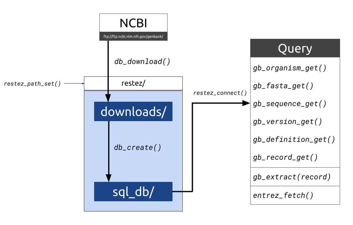
Here, we will do the following:
- Specify a location for our database (
restez_path) - Download the smallest section of GenBank (unannotated)
- Build a local database
# CODE

library(restez)
#> -------------
#> restez v1.0.2
#> -------------
#> Remember to restez_path_set() and, then, restez_connect()
# 1. Set the filepath for where the database will be stored
rstz_pth <- file.path(tempdir(), 'unannotated_database')
if (!dir.exists(rstz_pth)) {
  dir.create(rstz_pth)
}
restez_path_set(filepath = rstz_pth)
# 2. Download
# select number 20, for unannoated (the smallest section)
db_download(preselection = '20')
# 3. Create database
# connect to empty database
restez_connect()
#> Remember to run `restez_disconnect()`
db_create()
# always disconnect from a database when not in use.
restez_disconnect()

# OUTPUT
#> ... Creating '/var/folders/ps/g89999v12490dmp0jnsfmykm0043m3/T//Rtmpbpcz4s/unannotated_database/restez'
#> ... Creating '/var/folders/ps/g89999v12490dmp0jnsfmykm0043m3/T//Rtmpbpcz4s/unannotated_database/restez/downloads'
#> ────────────────────────────────────────────────────────────────────────────────────
#> Looking up latest GenBank release ...
#> ... release number 234
#> ... found 2539 sequence files
#> ────────────────────────────────────────────────────────────────────────────────────
#> Which sequence file types would you like to download?
#> Choose from those listed below:
#> ● 1  - 'EST (expressed sequence tag)'
#>         574 files and 243 GB
#> ● 2  - 'Bacterial'
#>         387 files and 168 GB
#> ● 3  - 'GSS (genome survey sequence)'
#>         268 files and 117 GB
#> ● 4  - 'Constructed'
#>         211 files and 88.6 GB
#> ● 5  - 'Patent'
#>         201 files and 84.1 GB
#> ● 6  - 'Plant sequence entries (including fungi and algae)'
#>         186 files and 93.1 GB
#> ● 7  - 'Other vertebrate'
#>         165 files and 68.2 GB
#> ● 8  - 'TSA (transcriptome shotgun assembly)'
#>         127 files and 53.9 GB
#> ● 9  - 'Invertebrate'
#>         110 files and 47.2 GB
#> ● 10 - 'HTGS (high throughput genomic sequencing)'
#>         82 files and 36.7 GB
#> ● 11 - 'Environmental sampling'
#>         58 files and 24.9 GB
#> ● 12 - 'Primate'
#>         34 files and 14.1 GB
#> ● 13 - 'Viral'
#>         34 files and 14.9 GB
#> ● 14 - 'Other mammalian'
#>         33 files and 9.57 GB
#> ● 15 - 'Synthetic and chimeric'
#>         27 files and 10.7 GB
#> ● 16 - 'Rodent'
#>         18 files and 7.41 GB
#> ● 17 - 'STS (sequence tagged site)'
#>         11 files and 4.45 GB
#> ● 18 - 'HTC (high throughput cDNA sequencing)'
#>         8 files and 3.45 GB
#> ● 19 - 'Phage'
#>         4 files and 1.52 GB
#> ● 20 - 'Unannotated'
#>         1 files and 0.00175 GB
#> Provide one or more numbers separated by spaces.
#> e.g. to download all Mammalian sequences, type: "12 14 16" followed by Enter
#>
#> Which files would you like to download?
#> ────────────────────────────────────────────────────────────────────────────────────
#> You've selected a total of 1 file(s) and 0.00175 GB of uncompressed data.
#> These represent:
#> ● 'Unannotated'
#>
#> Based on stated GenBank files sizes, we estimate ...
#> ... 0.00035 GB for  compressed, downloaded files
#> ... 0.00214 GB for the SQL database
#> Leading to a total of 0.00249 GB
#>
#> Please note, the real sizes of the database and its downloads cannot be
#> accurately predicted beforehand.
#> These are just estimates, actual sizes may differ by up to a factor of two.
#>
#> Is this OK?
#> ────────────────────────────────────────────────────────────────────────────────────
#> Downloading ...
#> ... 'gbuna1.seq' (1/1)
#> Done. Enjoy your day.
#> Adding 1 file(s) to the database ...
#> ... [32m'gbuna1.seq.gz'[39m ([34m1/1[39m)
#> Done.We can send queries to the database using two different methods: restez functions or rentrez wrappers.
What is
rentrez? Therentrezpackage allows users to interact with NCBI Entrez.restezwraps around some of its functions so that instead of sending queries across the internet, the local database is checked first.
# CODE

# import library, point to database and connect
library(restez)
rstz_pth <- file.path(tempdir(), 'unannotated_database')
restez_path_set(filepath = rstz_pth)
restez_connect()
#> Remember to run `restez_disconnect()`
# Check the status
restez_status()
# Get a random ID from the database
id <- sample(x = list_db_ids(n = 100), size = 1)
#> Warning in list_db_ids(n = 100): Number of ids returned was limited to [100].
#> Set `n=NULL` to return all ids.
# print record information
record <- gb_record_get(id)
cat(record)
# see ?gb_record_get for more query functions
# always disconnect
restez_disconnect()

# OUTPUT
#> Checking setup status at  ...
#> ────────────────────────────────────────────────────────────────────────────────────
#> Restez path ...
#> ... Path '/var/folders/ps/g89999v12490dmp0jnsfmykm0043m3/T//Rtmpbpcz4s/unannotated_database/restez'
#> ... Does path exist? 'Yes'
#> ────────────────────────────────────────────────────────────────────────────────────
#> Download ...
#> ... Path '/var/folders/ps/g89999v12490dmp0jnsfmykm0043m3/T//Rtmpbpcz4s/unannotated_database/restez/downloads'
#> ... Does path exist? 'Yes'
#> ... N. files 2
#> ... N. GBs 0
#> ... GenBank division selections 'Unannotated'
#> ... GenBank Release 234
#> ... Last updated '2019-11-07 20:08:38'
#> ────────────────────────────────────────────────────────────────────────────────────
#> Database ...
#> ... Path '/var/folders/ps/g89999v12490dmp0jnsfmykm0043m3/T//Rtmpbpcz4s/unannotated_database/restez/sql_db'
#> ... Does path exist? 'Yes'
#> ... N. GBs 0
#> ... Is database connected? 'Yes'
#> ... Does the database have data? 'Yes'
#> ... Number of sequences 543
#> ... Min. sequence length 0
#> ... Max. sequence length Inf
#> ... Last_updated '2019-11-07 20:08:45'
#> LOCUS       SCAF000130               299 bp    RNA     linear   UNA 15-MAY-1997
#> DEFINITION  Synthetic RNA ligase ribozyme CM2g, complete sequence.
#> ACCESSION   AF000130
#> VERSION     AF000130.1
#> KEYWORDS    .
#> SOURCE      unidentified
#>   ORGANISM  unidentified
#>             unclassified sequences.
#> REFERENCE   1  (bases 1 to 299)
#>   AUTHORS   Hager,A.J. and Szostak,J.W.
#>   TITLE     Isolation of novel ribozymes that ligate AMP-activated RNA
#>             substrates
#>   JOURNAL   Unpublished
#> REFERENCE   2  (bases 1 to 299)
#>   AUTHORS   Hager,A.J. and Szostak,J.W.
#>   TITLE     Direct Submission
#>   JOURNAL   Submitted (17-APR-1997) Molecular Biology, MGH, Boston, MA 02114,
#>             USA
#> FEATURES             Location/Qualifiers
#>      source          1..299
#>                      /organism="unidentified"
#>                      /mol_type="genomic RNA"
#>                      /db_xref="taxon:32644"
#>                      /note="ligase ribozyme CM2g"
#> ORIGIN
#>         1 ggcaacgcgc gactaggata ggcacctcag agagtggcca aacagttcgg gggaagatgc
#>        61 cgtgtagtat ggccagggga agtatagctg ccgcgacacg atgtcccgag ccagcaaccc
#>       121 agtgatctta ttgaggtgat caccagtgtc tacattcgat gtatgacgcg ttgggaagaa
#>       181 actctggcac cgttgccgac tagggtggcc attaatacct caggcccacc gaagcatggg
#>       241 gacaccagtg tcgccgatcg accatacttc ccgagaccgt atagcctgtc cttagatac
#> //
outsider is a package that allows users to install and run external code within the R environment. This is very useful when trying to construct pipelines that make use of a variety of code. outsider requires Docker to work. It should be able to launch any (?!) command-line program.
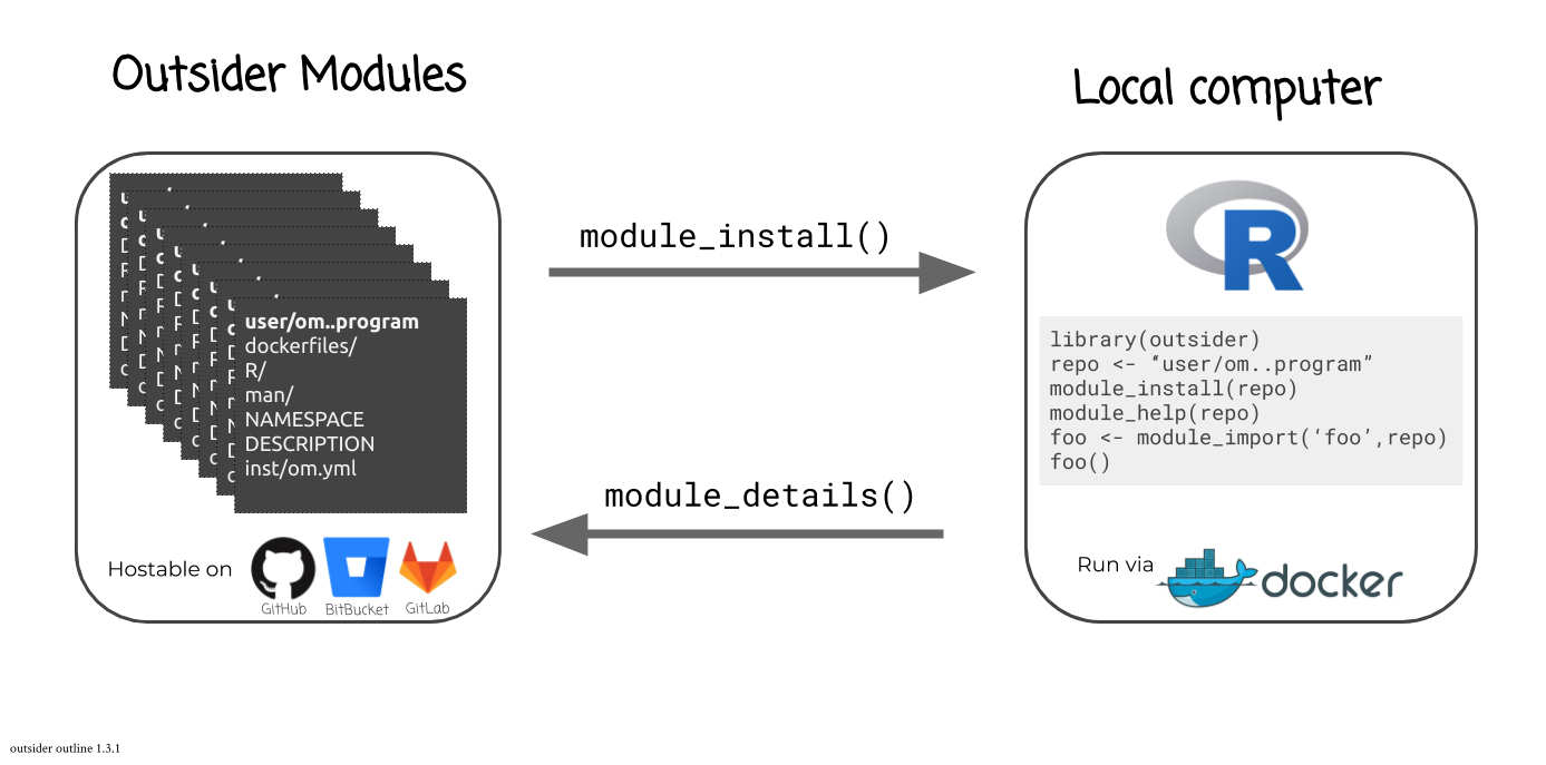
You can find out what modules are available for a given coding-service using:
library(outsider)
module_details(service = 'github')
#> Warning in FUN(X[[i]], ...): Unable to fetch data from GitHub for
#> 'hrbrmstr/om..nmap'
#> # A tibble: 16 x 7
#>    repo   program details versions updated_at          watchers_count url
#>    <chr>  <chr>   <chr>   <chr>    <dttm>                       <int> <chr>
#>  1 DomBe… PyRate  Estima… latest,… 2019-10-25 13:06:00              1 http…
#>  2 hrbrm… ""      ""      ""       2019-03-23 17:02:00              1 http…
#>  3 DomBe… pyphla… TODO w… latest   2019-10-31 17:08:00              0 http…
#>  4 DomBe… wikit   Fetch … latest   2019-10-25 15:27:00              0 http…
#>  5 DomBe… RAxML   Random… latest   2019-10-25 14:21:00              0 http…
#>  6 DomBe… beast   Bayesi… latest   2019-10-25 13:07:00              0 http…
#>  7 DomBe… astral  Accura… latest   2019-10-25 13:07:00              0 http…
#>  8 DomBe… revbay… Bayesi… latest   2019-10-25 13:06:00              0 http…
#>  9 DomBe… BAMM    Bayesi… latest,… 2019-10-25 13:05:00              0 http…
#> 10 DomBe… blast   Basic … latest,… 2019-10-25 13:01:00              0 http…
#> 11 DomBe… trimal  A tool… latest   2019-10-25 12:59:00              0 http…
#> 12 DomBe… pasta   PASTA … latest   2019-10-25 12:58:00              0 http…
#> 13 DomBe… Partit… Partit… latest   2019-10-25 12:58:00              0 http…
#> 14 DomBe… mafft   Multip… latest   2019-10-25 12:57:00              0 http…
#> 15 DomBe… figlet  ASCII … latest   2019-10-24 15:09:00              0 http…
#> 16 DomBe… hello … Templa… latest   2019-08-19 09:30:00              0 http…
There is also a package called "outsider.devtools" that makes it easier to create your own moduules, see other/outsider_devtools.R
To demonstrate, let's run an alignment software tool, mafft, from within R. Let's install a module for mafft, and then run it on some test sequences ("ex_seqs.fasta").
# CODE

library(outsider)
# squelch text to console
verbosity_set(show_program = FALSE, show_docker = FALSE)
# github repo to where the module is located
repo <- 'dombennett/om..mafft'
# install mafft
module_install(repo = repo, force = TRUE)
# look up available functions
(module_functions(repo = repo))
# import mafft function
mafft <- module_import(fname = 'mafft', repo = repo)
# test function
mafft(arglist = '--help')

# OUTPUT
#> [1] "mafft"library(outsider)
# Use example mafft nucleotide data
ex_seqs_file <- file.path(getwd(), 'data', 'ex_seqs.fasta')
(file.exists(ex_seqs_file))
# Run
mafft <- module_import(fname = 'mafft', repo = 'dombennett/om..mafft')
ex_al_file <- file.path(getwd(), 'data', "ex_al.fasta")
mafft(arglist = c('--auto', ex_seqs_file, '>', ex_al_file))
(file.exists(ex_al_file))
# View alignment
cat(readLines(con = ex_al_file, n = 50), sep = '\n')
#> [1] TRUE
#> [1] TRUE
#> >X02729 Methanococcus vannielli. #
#> ----tatctattaccctacc----ctggggaatggcttggcttgaaacgccgatgaagga
#> cgtggtaagctgcgataagcctaggcgaggcgcaa-cagcctttgaacctaggatttccg
#> aatgggacttcctacttttgtaa--------------------tccgtaaggattggtaa
#> cgcgggggattgaagcatcttagtacccgcaggaaaagaaatca-actgaga-ttccgtt
#> agtagaggcgattgaacacggatcagggcaaactgaatcccttcg-------------gg
#> gagatgtggtgttatagggccttct------tttcgcctgttgagaaaagctgaagtt-g
#> actggaacg-tcacactatagagggtgaaagtcccgtaagcgcaatcgattcaggtt---
#> tgaagtgt-ccctgagtaccgtgcgttggatatcgcgcgggaatt-tgggaggcatcaac
#> ttccaactctaaatacgtttcaagaccgatagcgtac-tagtaccgcgagggaaagctga
#> aaagcacccttaacagggtggtgaaa-agagcctgaaacccaggtaggtatggaatggcg
#> tggccccaaagg-----caactgttctgaaggaaaccgtcgcaaggcggctgtacgaaga
#> acag---agccagggttgcgtcctccgtttcgaaaaacgggccggggagtgta-ttgttg
#> tggcgagcttaagatcttcac--gatcgaaggcgtagggaaaccaacaagtccgcagaat
#> ct---------ttagggacggggtctt--aagggcccggagtcacagcaatacgacccga
#> aaccgggcgatctaggccggggcaaggtgaagtccctcaattgagggatggaggcctg-c
#> agagttgttgccgttcgaagcactcttctgacctcggtctaggggtgaaaggccaatcga
#> gcccggagatagctggttcccctcgaagtgactctcaggtcagccagagttcaggtagtc
#> ggcagggtagagc-actgataagatggttag-----gggaagaaattcctcgctgttttg
#> tcaaactccgaacctgtcgtcgccg-taggctctgagtga-gggcatacggggtaagctg
#> tatgtccgagacgggaatagccgagacttgggttaaggcccctaaatgccgattaagtgt
#> gaac---acgaagggcgtccttggtctaagacagcagggaggttggcttagaagcagcca
#> ccctttaaagagtgcgtaacagctcacctgtcgagatcaagggccccgaaaatggacggg
#> gct-aaatcggctgccgagacccaaagggcaccgcaag--------gtgatccccgtagg
#> ggggcgttctgcgagggcagaagttcggctgtgaagtcgagtggacctcgtagaaatgaa
#> gatcccggtagtagtaacagcataagtggggtgagaa-tccccaccgccgaaggggcaag
#> ggttccacagcaatgtttgtcagctgtgggtaagccggtcctaactctcgaggtaa--ct
#> cctttgagaggaa-agggaaacaggttaatattcctgtgc------catctagatacgcg
#> tggcaacacaaggttagt-ttccaacgcttctgggtaggctgagtgtt-cttgtctggac
#> attcaagcttataag-tccggggagagttgtaataacgagaaccg-gatgaaagagtgat
#> gagct-ctccgttaggagagttcggccgatctctggagcccgtgaaaagggaactagca-
#> -aggattctagatgtccgtacccagaaccgacactggtgcccctaggtgagtatcctaag
#> gcgtagcgggatgaatctagtcgagggaagtcggcaaattggttccgtaacttcgggaga
#> aggagtgccagtgatcttgtttaaatatgggatcgctggtcgcagtgaccagggaggtcc
#> gactgtttaatacaaacataggtcttagcgagcctgaaaaggtgtgtactaaggccgacg
#> cctgcccagtgctggtacgtgaaccccggttccaaccgggcgaagcgccagtaaacggcg
#> ggggtaactataaccctcttaaggtagcgaaattccttgtcgggcaagttccgacctgca
#> tgaatggcgtaacgagacctccactgtccccgactagaatccggtgaacctaccattccg
#> gcgcaaag-gccggagacttccagtgggaagcgaagaccccgtggagctttactgcagcc
#> tgtcgttggggcatggttgtgagtgtacagtgtaggtgggagccatcgaaaccttttcgc
#> c----aggaaaggtggaggcgatcctgggacaccaccctctcatgaccatgttcctcacc
#> ctt-----ttaggggacaccggtaggtgggcagtttggctggggcggtaccctcctaaaa
#> atgcatcaggagggccccaaaggttggctcaagcgggtcaggactccgctgttgagtg-t
#> aagggcaaaagccagcctgactttgttgccaacaaaacg-caacgaagaggcgaaagccg
#> ggcctaacgaacccctgtg--cctcactgatgggggccagggatgacaaaaaagctaccc
#> cggggataacagagttgtcgcgggcaagagcccatatcgaccccgcggcttgctacctcg
#> atgtcggtttttcccatcctgggtctgcagcaggacccaagggtggggctgttcgcccat
#> taaaggggatcatgagctgggtttagaccgtcgtgagacaggttggttgctatctgctgg
#> atgtgttaggctgtctgagggaaaggtggctctagtacgagaggaacgggccgtcggcgc
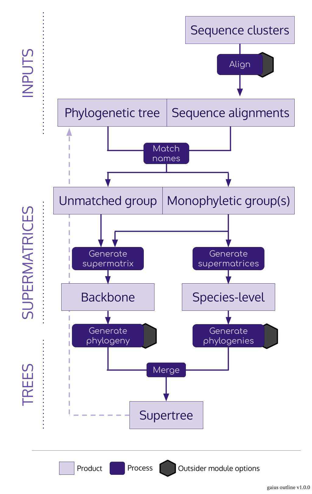
#> ctctagtcgatcggttgtctgacaaggcac-tgccgagcagccacgcgccaagaga-taagaiusacts as the nexus package for the SUPERSMART pipeline in R- It imports both alignments and trees and produces supermatrices and supertrees
- Its main role is to identify monophyletic groups of a given number of taxa for species-level trees
- The main "trick" is to use a pre-existing tree
- It can do a few clever things: there can be any number of levels of backbone, backbone supermatrices are constucted from an assortment of the best monophyletic sequences
# CODE

library(gaius)
# vars
alignment_dir <- file.path(getwd(), 'data', 'gaius_alignments')
tree_file <- file.path(getwd(), 'data', 'taxtree.tre')
# alignment files
alignment_files <- file.path(alignment_dir,
                             list.files(path = alignment_dir,
                                        pattern = '.fasta'))
(alignment_files[1:2])
# get alignment names
alignment_names <- names_from_alignments(alignment_files)
(alignment_names[1:10])
# tree tip names
tree_names <- names_from_tree(tree_file)
(tree_names[1:10])
# match alignment names to those in tree
matched_names <- name_match(alignment_names = alignment_names,
                            tree_names = tree_names)
(matched_names)
# identify monophyletic groups
groups <- groups_get(tree_file = tree_file, matched_names = matched_names)
(groups)
# read in alignments
alignment_list <- alignment_read(flpths = alignment_files)
(alignment_list)
# ^ for a better idea of the alignment, try ...
# viz(alignment_list[[1]])
# construct supermatrices
supermatrices <- supermatrices_get(alignment_list = alignment_list,
                                   groups = groups, min_ngenes = 2,
                                   min_ntips = 3, min_nbps = 100,
                                   column_cutoff = 0, tip_cutoff = 0.1)
(supermatrices)

# OUTPUT
#> [1] "/Users/djb208/Coding/supersmartR-workshop-mini/data/gaius_alignments/11_cluster_alignment.fasta"
#> [2] "/Users/djb208/Coding/supersmartR-workshop-mini/data/gaius_alignments/9_cluster_alignment.fasta"
#>  [1] "Hystrix_brachyura"
#>  [2] "Cavia_tschudii"
#>  [3] "Galea_musteloides"
#>  [4] "Hydrochoerus_hydrochaeris"
#>  [5] "Myocastor_coypus"
#>  [6] "Aconaemys_sagei"
#>  [7] "Octodon_bridgesi"
#>  [8] "Tympanoctomys_loschalchalerosorum"
#>  [9] "Dactylomys_boliviensis"
#> [10] "Dactylomys_dactylinus"
#>  [1] "Abrocoma_bennettii_bennettii" "Abrocoma_boliviensis"
#>  [3] "Abrocoma_cinerea"             "Aconaemys_fuscus"
#>  [5] "Aconaemys_porteri"            "Aconaemys_sagei"
#>  [7] "Atherurus_africanus"          "Atherurus_macrourus"
#>  [9] "Bathyergus_janetta"           "Bathyergus_sp_CAM_2005"
#> [141] names matched:
#> ... from `$alignment` Hystrix_brachyura, Cavia_tschudii, Galea_musteloides ...
#> ... to `$tree` Hystrix_brachyura_hodgsoni, Cavia_tschudii_osgoodi, Galea_musteloides_leucoblephara ...
#> [0] unmatched.
#> Tips group object of [7] elements:
#> ... [114] tips in mono
#> ... [27] tips in super'alignment_list' object, with 4 'alignment' objects
#>
#> [["11_cluster_alignment"]] ...
#> An 'alignment': 62 tips x 1102 bps
#> ... $Hystrix_brachyura                 --------gactacctaaacggccccttcaccg ...
#> ... $Cavia_tschudii                    --------gattacctaaatggtcccttcacag ...
#> ... $Galea_musteloides                 --------gactacctcaatggccccttcacgg ...
#> ... $Hydrochoerus_hydrochaeris         --------gactacctaaatggccccttcacgg ...
#> ... $Myocastor_coypus                  --------gattacctcaatggccccttcacgg ...
#> ... $Aconaemys_sagei                   --------gactacctnaanggccccttcacgg ...
#> ... $Octodon_bridgesi                  --------gactacctcaatggccccttcacgg ...
#> ... $Tympanoctomys_loschalchalerosorum --------gactacctcaatggtcccttcacgg ...
#> ... $Dactylomys_boliviensis            accttgacgtcatcatcaacgggcacttcacgg ...
#> ... $Dactylomys_dactylinus             accttgatgactacctcaacggccccttcatgg ...
#> ... with 52 more tip(s)
#>
#> ... [["genegrowth_alignment"]]
#> 'supermatices' list, with 7 'supermatrix' objects
#>
#> [["n88"]] ...
#> A 'supermatrix': 6 tips x 5227 bps x 4 genes, 64% gaps
#> ... $Octodontomys_gliroides --------gactacctcaatggccccttcacggtggtggtcaag ...
#> ... $Ctenomys_boliviensis   -------------cctcaatggccccttcacggtggtggtcaag ...
#> ... $Ctenomys_coyhaiquensis accttgatgactacctcaatggccccttcacggtggtggtcaag ...
#> ... $Ctenomys_minutus       accttgacgactacctcaatggccccttcgcggtggtggtcaag ...
#> ... $Ctenomys_haigi         -------------------------------------------- ...
#> ... $Ctenomys_steinbachi    -------------------------------------------- ...
#>
#> ... [["backbone"]]
A complete pipeline for constructing a phylogenetic tree of all Caviomorpha species is contained in pipeline/. The pipeline uses the above packages and their functions. We can run each script of the pipeline using source(). (To save time we will skip the restez and phylotaR steps and download a completed folder of the first part of the results.)
## Code

# minor outsider set-up
if (file.exists('gc_setup.R')) {
  source(file = 'gc_setup.R', local = FALSE, echo = FALSE, print.eval = FALSE)
} else {
  threads <- 4
}
#> Remember to run ssh_teardown() when finished.

# save time by skipping the first two stages by using the ready
#  1_phylotaR/ in data/
zipfile <- file.path('data', '1_phylotaR.zip')
if (file.exists(zipfile)) {
  utils::unzip(zipfile = zipfile, exdir = 'pipeline', overwrite = TRUE)
}

# run each script in the pipeline
stage_scripts <- c('2_clusters.R', '3_align.R', '4_supermatrix.R',
                   '5_phylogeny.R', '6_supertree.R', '7_view.R')
start_time <- Sys.time()
cat('Running pipeline ....\n', sep = '')
for (stage_script in stage_scripts) {
  cat('... ', crayon::green(stage_script), '\n', sep = '')
  scriptenv <- new.env()
  scriptenv$threads <- threads
  suppressMessages(source(file.path('pipeline', stage_script),
                          local = scriptenv, echo = FALSE, print.eval = FALSE))
}
end_time <- Sys.time()
duration <- difftime(end_time, start_time, units = 'mins')
cat('Duration: ', crayon::red(round(x = duration, digits = 3)), ' minutes.\n')

# clear-up
outsider::ssh_teardown()

## Output
#> Running pipeline ....
#> ... 2_clusters.R
#> ... 3_align.R
#> ... ... aligning  10_cluster
#> ... ... aligning  11_cluster
#> ... ... aligning  14_cluster
#> ... ... aligning  15_cluster
#> ... ... aligning  16_cluster
#> ... ... aligning  17_cluster
#> ... ... aligning  18_cluster
#> ... ... aligning  3_cluster
#> ... ... aligning  6_cluster
#> ... ... aligning  8_cluster
#> ... ... aligning  9_cluster
#> ... ... aligning  barcode
#> ... ... aligning  cytochrome
#> ... ... aligning  factorvwf
#> ... ... aligning  gene
#> ... ... aligning  genegrowth
#> ... 4_supermatrix.R
#> ... 5_phylogeny.R
#> ... ... generating tree for  backbone
#> ... ... generating tree for  n211
#> ... ... generating tree for  n224
#> ... ... generating tree for  n276
#> ... ... generating tree for  n340
#> ... ... generating tree for  n375
#> ... ... generating tree for  n88
#> ... 6_supertree.R
#> ... 7_view.R
#> Duration:  5.292  minutes.
The resulting tree consists of 185 tips, generating from 16 gene/clusters.

Learn more: supersmartR GitHub Page