Agentic systems, whether designed for tool use or for reasoning, are fundamentally built on prompts. Yet prompts themselves follow a linear, sequential pattern and cannot self-optimize. Real agentic training comes from the way an agent learns, adapts, and collaborates in dynamic environments.
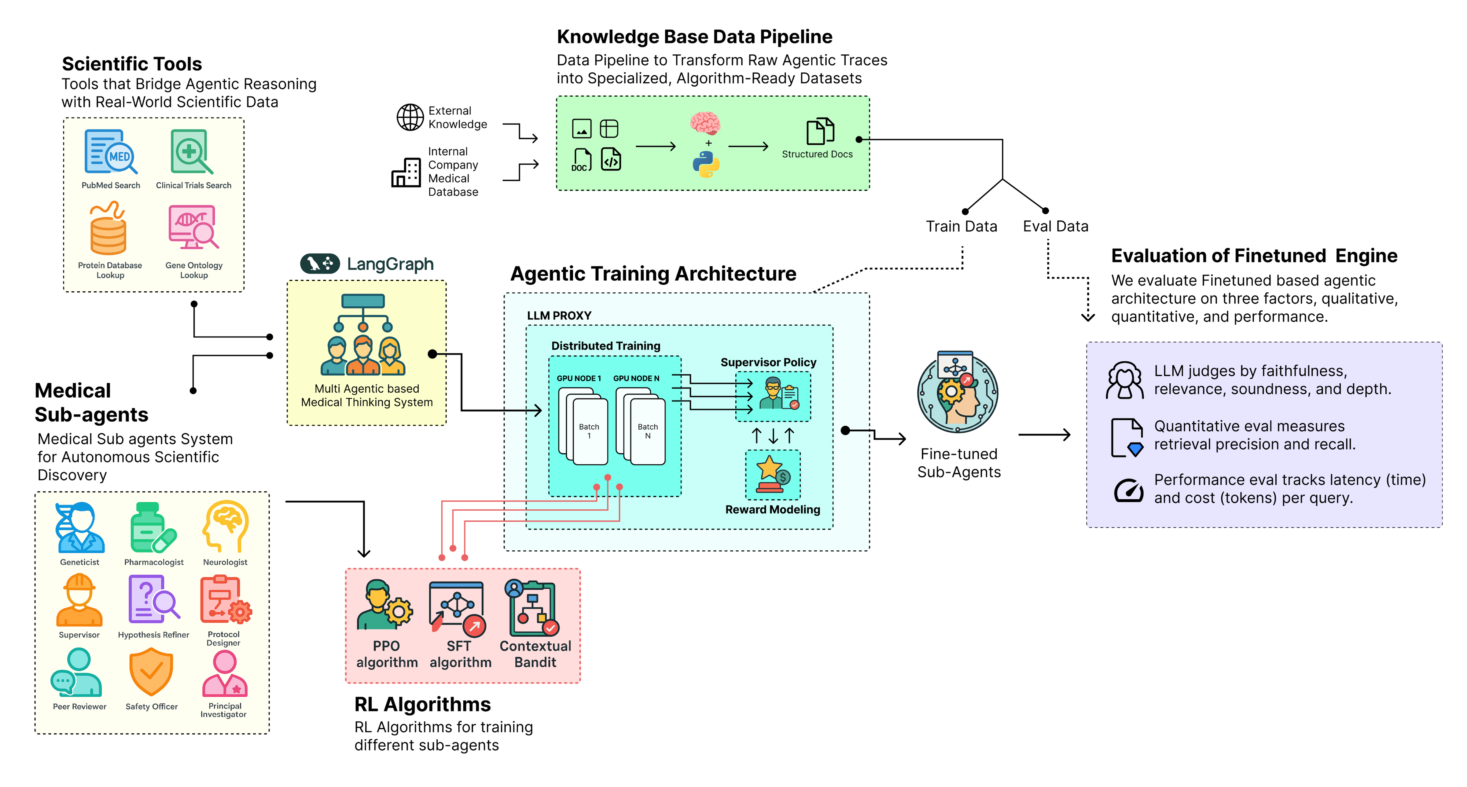
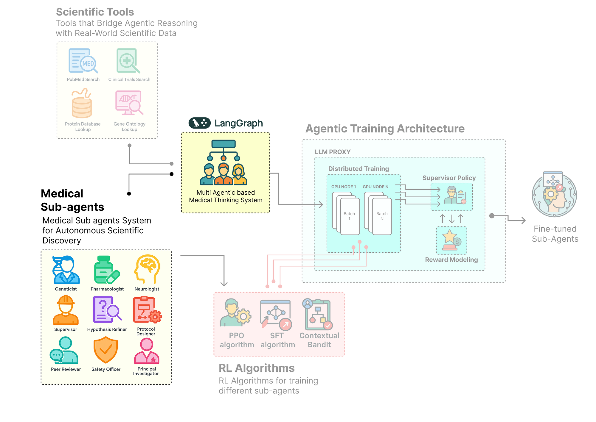
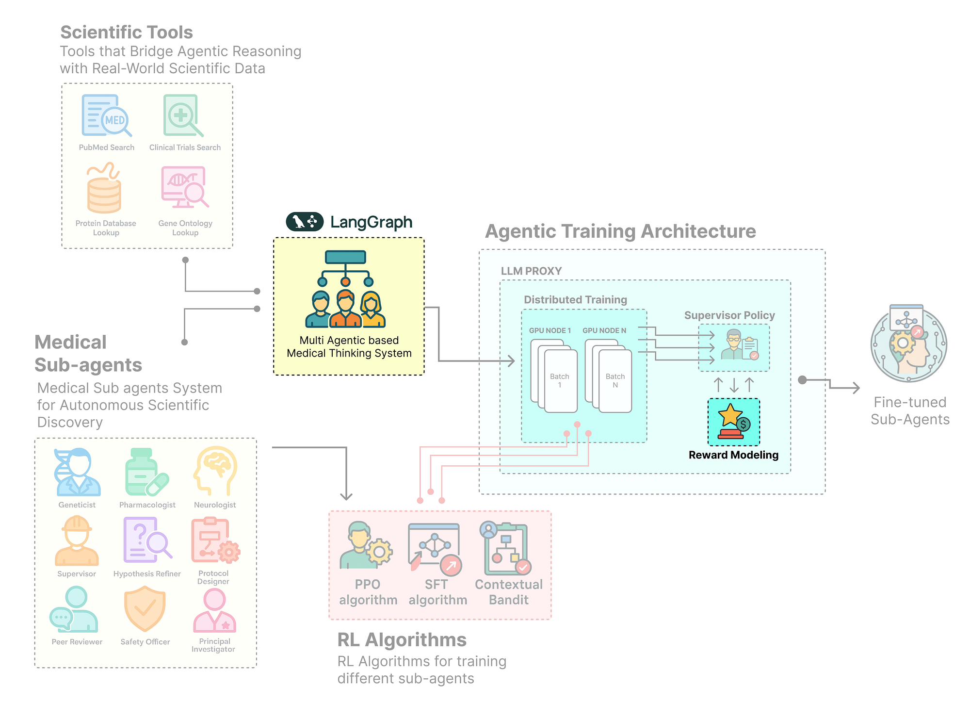
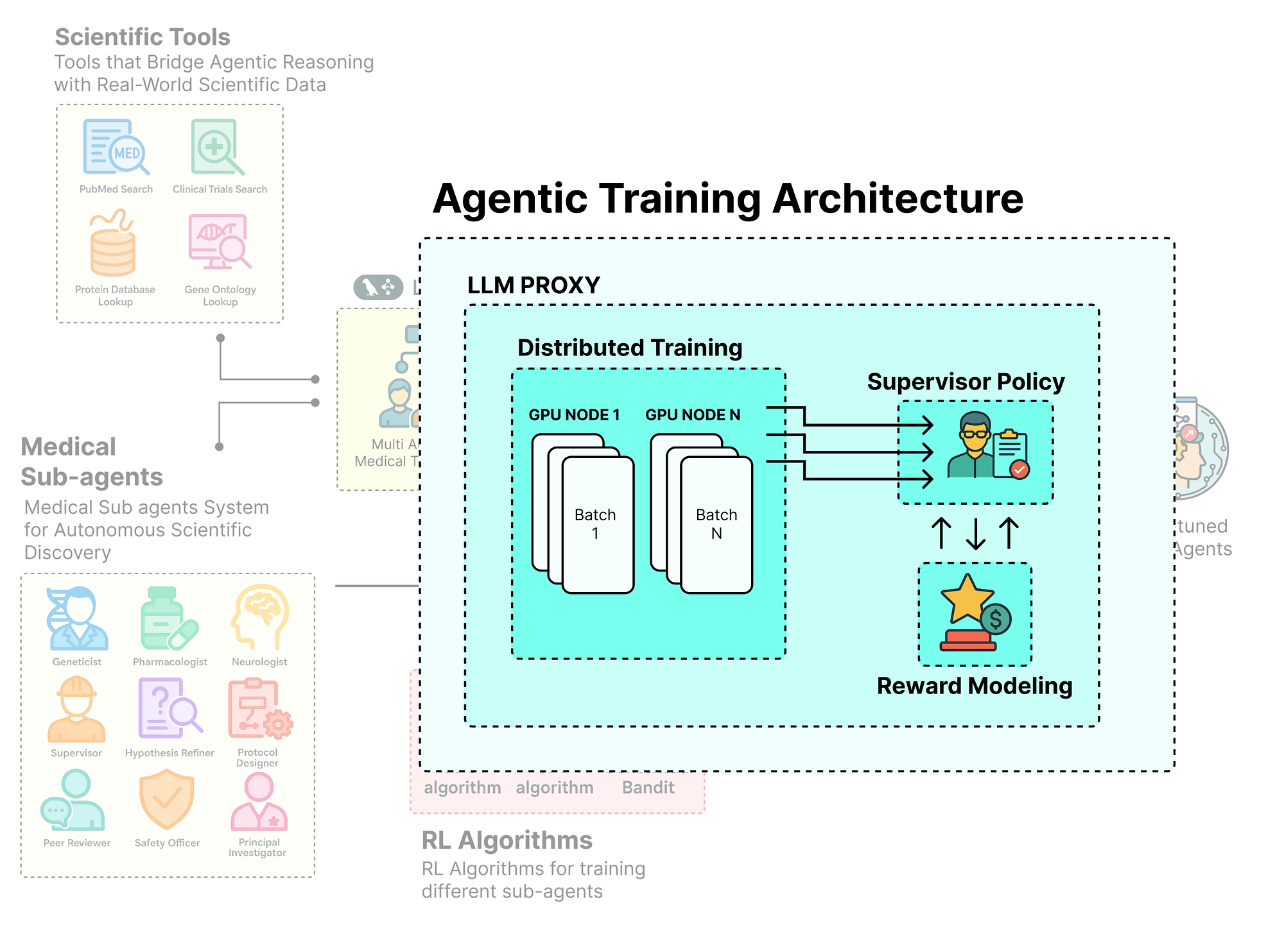
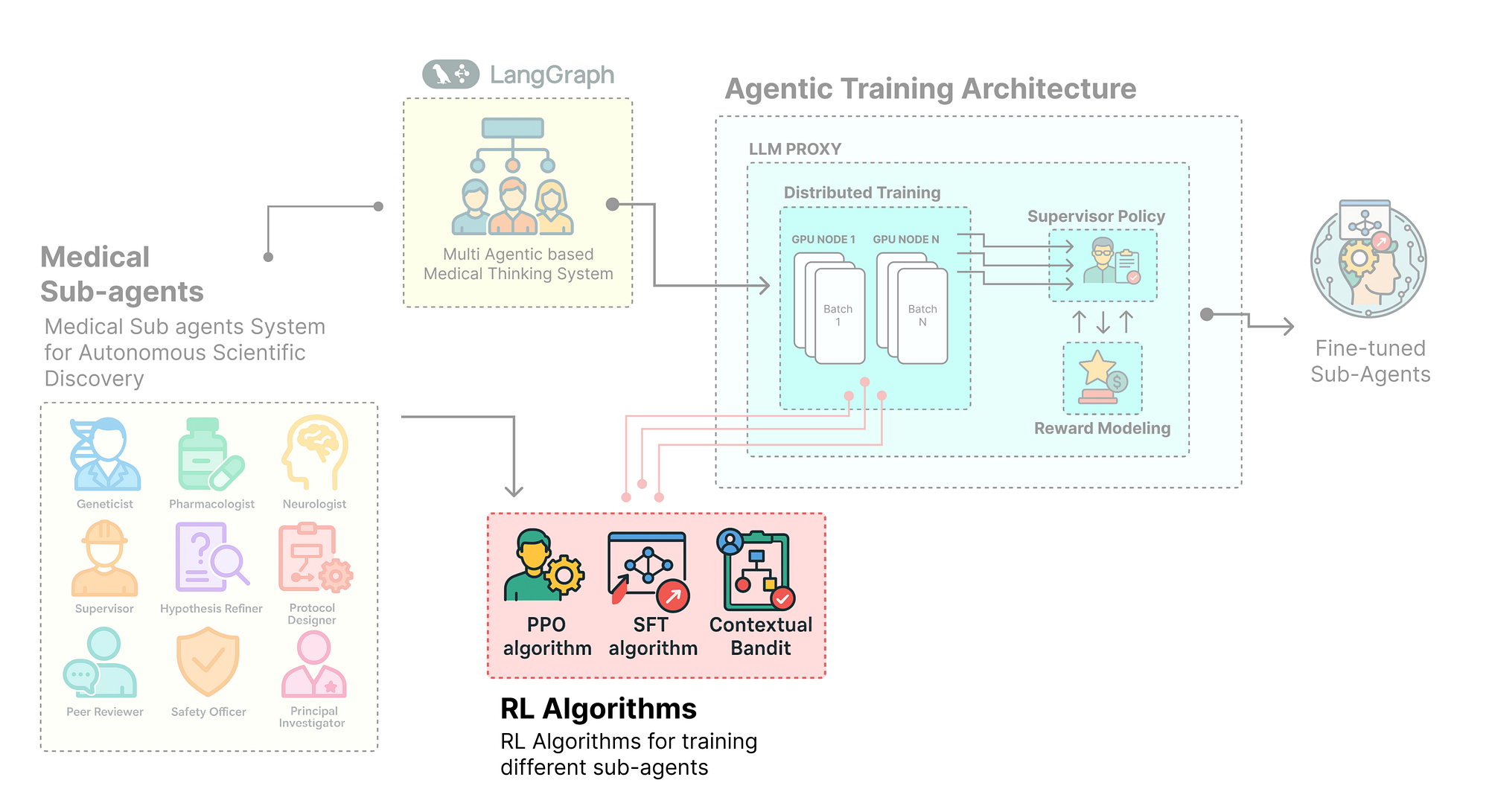
In an agentic architecture each sub-agent has a different purpose, and that means a single algorithm won’t work for all. To make them more effective, we need a complete training architecture that connects reasoning, reward, and real-time feedback. A typical training architecture for an agentic system involves several interconnected components …
- First, we define the training foundation by setting up the environment, initializing agent states, and aligning their objectives with the system goals.
- Next, we build the distributed training pipeline where multiple agents can interact, learn in parallel, and exchange knowledge through shared memory or logs.
- We add the reinforcement learning layer that powers self-improvement using algorithms like SFT for beginners, PPO for advanced optimization, and contextual bandits for adaptive decision making.
- We connect observability and monitoring tools such as tracing hooks and logging adapters to capture every interaction and learning step in real time.
- We design a dynamic reward system that allows agents to receive feedback based on their performance, alignment, and contribution to the overall task.
- We create a multi phase training loop where agents progress through different stages, from supervised fine tuning to full reinforcement based adaptation.
- Finally, we evaluate and refine the architecture by analyzing reward curves, performance metrics, and qualitative behavior across all agent roles.
In this blog we are going to …
build a complete multi-agentic system combining reasoning, collaboration, and reinforcement learning (RL) to enable agents to adapt and improve through real-time feedback and rewards.
- Creating the Foundation for an Research Lab
- Designing Our Society of Scientists (LangGraph)
- Creating the RL Based Training Architecture
- Implementing Three RL Algorithms
- Building the 3 Phases based Training Loop
- Performance Evaluation and Analysis
- How Our RL Training Logic Works
When we start building a production-grade AI system we don’t instantly start with the algorithm, but with a proper foundation of the entire system. This initial setup is important every choice we make here from the libraries we install to the data we source, will determine the reliability and reproducibility of our final trained agent.
So, in this section this is what we are going to do:
- We are going to install all core libraries and specialized dependencies required for our hierarchical training setup.
- Then we we are going to perform configurtion of our API keys, avoiding hardcoded values, and connect our LangSmith project for observability.
- After configurtion, we are going to download and process the PubMedQA dataset to build a high-quality corpus for our agents.
- We are also going to design the central AgentState, the shared memory that enables collaboration and reasoning.
- Then going to equip our agents with essential tools such as mock databases, live web search and more for external interaction.
First, we need to set up our Python environment. Instead of a simple pip install, we are going to use uv, because it’s is not a fast and modern package manager, to ensure our environment is both quick to set up and highly reproducible suitable for production environment.
We are also installing specific extras for agent-lightning verl for our PPO algorithm and apo (Asynchronous Policy Optimization) and unsloth for efficient SFT which are important for our advanced hierarchical training strategy.
print("Updating and installing system packages...")
# We first update the system's package list and install 'uv' and 'graphviz'.
# 'graphviz' is a system dependency required by LangGraph to visualize our agentic workflows.
!apt-get update -qq && apt-get install -y -qq uv graphviz


print("\nInstalling packages...\n")
# Here, we use 'uv' to install our Python dependencies.
# We install the '[verl,apo]' extras for Agent-Lightning to get the necessary components for PPO and other advanced RL algorithms.
# '[unsloth[pt231]]' provides a highly optimized framework for Supervised Fine-Tuning, which we'll use for our Junior Researchers.
!uv pip install -q -U "langchain" "langgraph" "langchain_openai" "tavily-python" "agentlightning[verl,apo]" "unsloth[pt231]" "pandas" "scikit-learn" "rich" "wandb" "datasets" "pyarrow"
print("Successfully installed all required packages.")
Let’ start the installation process …
#### OUTPUT ####
Updating and installing system packages...
...
Installing packages...
Resolved 178 packages in 3.12s
...
+ agentlightning==0.2.2
+ langchain==0.2.5
+ langgraph==0.1.5
+ unsloth==2024.5
+ verl==0.6.0
...
Successfully installed all required packages.
By installing graphviz, we have enabled the visualization capabilities of LangGraph, which will be invaluable for debugging our complex agent society later.
More importantly, the installation of agentlightning with the verl and unsloth extras gives us the specific, high-performance training backends we need for our hierarchical strategy.
We now have a stable and complete foundation to build upon. We can now start pre-processing the training data.
Every machine learning system requires training data or at least some initial observations to begin self-learning.
Our agents cannot reason in isolation they need access to rich, domain-specific information.
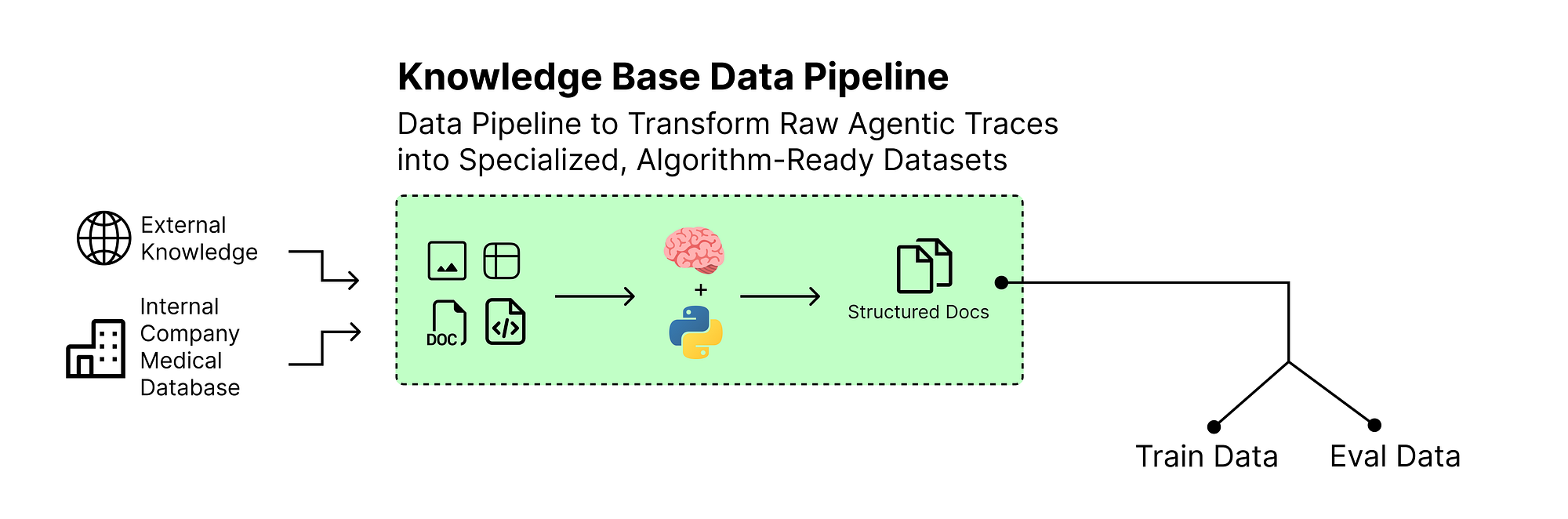
A static, hardcoded list of facts would be overly simplistic. To build a realistic and challenging research environment, we will draw our knowledge base from the PubMedQA dataset, specifically utilizing its labeled subset, pqa_l.
It contains real biomedical questions, the original scientific abstracts that provide the necessary context, and a final ‘yes/no/maybe’ answer determined by human experts. This structure provides not only a rich source of information for our agents to search but also a ground truth that we can use to calculate a reward for our reinforcement learning loop.
First, let’s define a simple TypedDict to structure each task. This ensures our data is clean and consistent throughout the pipeline.
from typing import List, TypedDict

# A TypedDict provides a clean, structured way to represent each research task.
# This makes our code more readable and less prone to errors from using plain dictionaries.
class ResearchTask(TypedDict):
    id: str                  # The unique PubMed ID for the article
    goal: str                # The research question our agent must investigate
    context: str             # The full scientific abstract providing the necessary evidence
    expected_decision: str   # The ground truth answer ('yes', 'no', or 'maybe')
We are basically creating a ResearchTask blueprint using TypedDict. This isn't just a plain dictionary, it's a contract that enforces a specific structure for our data. Every task will now consistently have an id, goal, context, and expected_decision. This strict typing is a best practice that prevents bugs down the line, ensuring that every component of our system knows exactly what kind of data to expect.
With our data structure defined, we can now write a function to download the dataset from the Hugging Face Hub, process it into our ResearchTask format, and split it into training and validation sets. A separate validation set is crucial for objectively evaluating our agent's performance after training.
from datasets import load_dataset
import pandas as pd

def load_and_prepare_dataset() -> tuple[List[ResearchTask], List[ResearchTask]]:
    """
    Downloads, processes, and splits the PubMedQA dataset into training and validation sets.
    """
    print("Downloading and preparing PubMedQA dataset...")
    # Load the 'pqa_l' (labeled) subset of the PubMedQA dataset.
    dataset = load_dataset("pubmed_qa", "pqa_l", trust_remote_code=True)
    # Convert the training split to a pandas DataFrame for easier manipulation.
    df = dataset['train'].to_pandas()

    # This list will hold our structured ResearchTask objects.
    research_tasks = []
    # Iterate through each row of the DataFrame to create our tasks.
    for _, row in df.iterrows():
        # The 'CONTEXTS' field is a list of strings; we join them into a single block of text.
        context_str = " ".join(row['CONTEXTS'])
        # Create a ResearchTask dictionary with the cleaned and structured data.
        task = ResearchTask(
            id=str(row['PUBMED_ID']),
            goal=row['QUESTION'],
            context=context_str,
            expected_decision=row['final_decision']
        )
        research_tasks.append(task)

    # We perform a simple 80/20 split for our training and validation sets.
    train_size = int(0.8 * len(research_tasks))
    train_set = research_tasks[:train_size]
    val_set = research_tasks[train_size:]

    print(f"Dataset downloaded and processed. Total samples: {len(research_tasks)}")
    print(f"Train dataset size: {len(train_set)} | Validation dataset size: {len(val_set)}")
    return train_set, val_set

# Let's execute the function.
train_dataset, val_dataset = load_and_prepare_dataset()
The load_and_prepare_dataset function we just coded is our data ingestion pipeline. It automates the entire process of sourcing our knowledge base: it connects to the Hugging Face Hub, downloads the raw data, and most importantly transforms it from a generic DataFrame into a clean list of our custom ResearchTask objects.
The 80/20 split is a standard machine learning practice, it gives us a large set of data to train on (
train_set) and a separate, unseen set (val_set) to later test how well our agent has generalized its knowledge.
Now that the data is loaded, it’s always a good practice to visually inspect a sample. This helps us confirm that our parsing logic worked correctly and gives us a feel for the kind of challenges our agents will face. We’ll write a small utility function to display a few examples in a clean, readable table.
from rich.console import Console
from rich.table import Table

console = Console()

def display_dataset_sample(dataset: List[ResearchTask], sample_size=5):
    """
    Displays a sample of the dataset in a rich, formatted table.
    """
    # Create a table for display using the 'rich' library for better readability.
    table = Table(title="PubMedQA Research Goals Dataset (Sample)")
    table.add_column("ID", style="cyan")
    table.add_column("Research Goal (Question)", style="magenta")
    table.add_column("Expected Decision", style="green")

    # Populate the table with the first few items from the dataset.
    for item in dataset[:sample_size]:
        table.add_row(item['id'], item['goal'], item['expected_decision'])

    console.print(table)

display_dataset_sample(train_dataset)
This display_dataset_sample function is our sanity check. By using the rich library to create a formatted table, we can quickly and clearly verify the structure of our loaded data. It's much more effective than just printing raw dictionaries. Seeing the data laid out like this confirms that our load_and_prepare_dataset function correctly extracted the ID, goal, and expected_decision for each task.
Let’s look at the output of the above function we have just coded.
#### OUTPUT ####
Downloading and preparing PubMedQA dataset...
Dataset downloaded and processed. Total samples: 1000
Train dataset size: 800 | Validation dataset size: 200

--- Sample 0 ---
ID: 11843333
Goal: Do all cases of ulcerative colitis in childhood need colectomy?
Expected Decision: yes
Context (first 200 chars): A retrospective review of 135 children with ulcerative colitis was performed to determin ...
sample_data (Created by Fareed Khan)
We have transformed the raw PubMedQA data into a clean, structured list of ResearchTask objects, split into training and validation sets. Each row in this table represents a complete research challenge that we can feed into our agent's rollout method.
The Research Goal will serve as the initial prompt, and the Expected Decision will be the ground truth for calculating our final reward signal. Our agents now have a world-class, realistic knowledge base to learn from.
With our data sourced and structured, we now need to design the “nervous system” of our agent society. This is the shared memory, or state, that will allow our diverse group of agents to collaborate, pass information, and build upon each other’s work. In LangGraph, this shared memory is managed by a central state object.
A simple dictionary would be too fragile for a complex system like ours. Instead, we will architect a nested, hierarchical
AgentStateusing Python'sTypedDict.
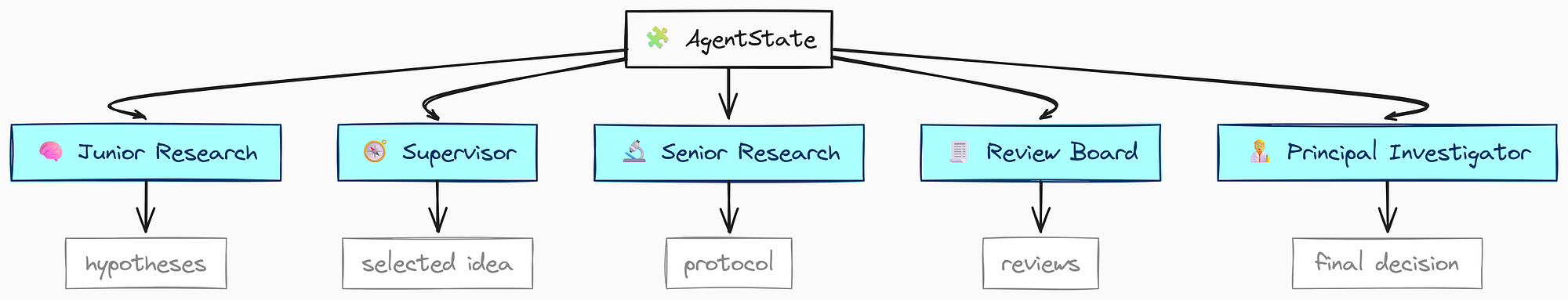
This approach provides a machine-readable blueprint for our agent entire cognitive process. Each field in our state will represent a distinct stage of the research workflow, from the initial hypotheses generated by the Junior Researchers to the final, peer-reviewed protocol.
Here’s what we are going to do:
- Define Sub-States: We will create smaller
TypedDictclasses for specific artifacts likeJuniorResearch,Protocol, andReviewDecision. - Architect the Master State: Assemble these sub-states into the main
AgentState, which will hold all information for a single research run. - Enable ReAct Logic: adding a
senderfield, a crucial component that allows us to build robust ReAct-style loops where tool results are routed back to the correct agent.
First, let’s define the data structure for the output from our Junior Researchers. This make sure that every hypothesis they generate is consistently formatted.
from typing import List, TypedDict, Literal
from langchain_core.messages import BaseMessage

# This defines the structure for a single hypothesis from a Junior Researcher.
# It captures the core idea, the evidence found, and which agent proposed it.
class JuniorResearch(TypedDict):
    hypothesis: str
    supporting_papers: List[str]
    agent_name: str # To track which junior researcher proposed it
We are basically creating a blueprint for what a “hypothesis submission” looks like. The JuniorResearch class uses TypedDict to enforce that every submission must contain a hypothesis string, a list of supporting_papers, and the agent_name. This structure is important for the Supervisor agent, as it guarantees it will receive a consistent set of proposals to evaluate, each with clear attribution.
Next, we will define the structure for the experimental protocol. This is the primary output of our Senior Researcher, and it needs to be detailed and actionable.
# This defines the structure for the final experimental protocol.
# It's a detailed, actionable plan.
class Protocol(TypedDict):
    title: str
    steps: List[str]
    safety_concerns: str
    budget_usd: float
The Protocol class formalizes the key components of a scientific experiment. By requiring a title, a list of steps, a safety_concerns section, and a budget_usd, we are instructing our Senior Researcher agent to think through the practical details of its proposal.
This structured output is far more valuable than a simple block of text and will be the basis for our final reward calculation.
Now, let’s create the structure for the feedback from our Review Board. This is crucial for our revision loop, as it needs to be both clear and machine-readable.
# This defines the structured feedback from our review agents.
# It forces a clear decision, a severity level, and constructive feedback.
class ReviewDecision(TypedDict):
    decision: Literal['APPROVE', 'REVISE']
    critique_severity: Literal['CRITICAL', 'MAJOR', 'MINOR']
    feedback: str
Here, we have designed the ReviewDecision class to capture the nuanced output of a critique. The use of Literal is a key piece of engineering:
- It forces the review agents to make a discrete choice (
APPROVEorREVISE) - To classify the severity of their feedback (
CRITICAL,MAJOR, orMINOR).
This way we are allowing our LangGraph router to decide whether to send the protocol back for a major rewrite or a minor tweak.
Finally, we can assemble these smaller structures into our main AgentState. This will be the single, comprehensive object that tracks everything that happens during a research run.
from typing import Annotated

# This is the master state dictionary that will be passed between all nodes in our LangGraph.
class AgentState(TypedDict):
    # The 'messages' field accumulates the conversation history.
    # The 'lambda x, y: x + y' tells LangGraph how to merge this field: by appending new messages.
    messages: Annotated[List[BaseMessage], lambda x, y: x + y]
    research_goal: str  # The initial high-level goal from our dataset.
    sender: str         # Crucial for ReAct: tracks which agent last acted, so tool results can be sent back to it.
    turn_count: int     # A counter to prevent infinite loops in our graph.

    # Junior Researcher Team's output (accumulates from parallel runs)
    initial_hypotheses: List[JuniorResearch]

    # Supervisor's choice
    selected_hypothesis: JuniorResearch
    supervisor_justification: str

    # Senior Researcher Team's output
    refined_hypothesis: str
    experimental_protocol: Protocol

    # Review Board's output
    peer_review: ReviewDecision
    safety_review: ReviewDecision

    # Principal Investigator's final decision
    final_protocol: Protocol
    final_decision: Literal['GO', 'NO-GO']
    final_rationale: str

    # The final evaluation score from our reward function
    final_evaluation: dict
We have now successfully defined the entire cognitive architecture of our agent society.
The flow of information is clear: initial_hypotheses are generated, one is chosen as the selected_hypothesis, it's refined into an experimental_protocol, it undergoes peer_review and safety_review, and results in a final_decision.
The sender field is particularly important.
In a ReAct (Reason-Act) loop, an agent decides to use a tool. After the tool runs, the system needs to know which agent to return the result to.
By updating the sender field every time an agent acts, we create a clear return address, enabling this complex, back-and-forth reasoning pattern. With this state defined, our graph now has a solid memory structure to work with.
Our agents now have a sophisticated memory (AgentState), but to perform their research, they need access to the outside world or in a more technical term (theexternal knowledgebase).
An agent without tools is just a conversationalist, an agent with tools becomes a powerful actor capable of gathering real-time, domain-specific information.
In this section, we will build a ScientificToolkit for our agent society. This toolkit will provide a set of specialized functions that our agents can call to perform essential research tasks.
Here is what we are going to do:
- Integrate Live Web Search: We will use the
TavilySearchResultstool to give our agents the ability to search PubMed and ClinicalTrials.gov for the latest scientific literature. - Simulate Internal Databases: We will create mock databases for proteins and gene ontologies to simulate how an agent would query proprietary, internal knowledge bases.
- Decorate with
@tool: Using LangChain@tooldecorator to make these Python functions discoverable and callable by our LLM-powered agents. - Test a Tool: Then to perform a quick test call on one of our new tools to ensure everything is wired up correctly.
First, let’s define the class that will house all our tools. Grouping them in a class is good practice for organization and state management (like managing API clients).
from langchain_core.tools import tool
from langchain_community.tools.tavily_search import TavilySearchResults


class ScientificToolkit:
    def __init__(self):
        # Initialize the Tavily search client, configured to return the top 5 results.
        self.tavily = TavilySearchResults(max_results=5)
        # This is a mock database simulating an internal resource for protein information.
        self.mock_protein_db = {
            "amyloid-beta": "A key protein involved in the formation of amyloid plaques in Alzheimer's.",
            "tau": "A protein that forms neurofibrillary tangles inside neurons in Alzheimer's.",
            "apoe4": "A genetic risk factor for Alzheimer's disease, affecting lipid metabolism in the brain.",
            "trem2": "A receptor on microglia that, when mutated, increases Alzheimer's risk.",
            "glp-1": "Glucagon-like peptide-1, a hormone involved in insulin regulation with potential neuroprotective effects."
        }
        # This is a second mock database, this time for gene functions.
        self.mock_go_db = {
            "apoe4": "A major genetic risk factor for Alzheimer's disease, involved in lipid transport and amyloid-beta clearance.",
            "trem2": "Associated with microglial function, immune response, and phagocytosis of amyloid-beta."
        }
We have now set up the foundation for our ScientificToolkit. Let’s quickly understand it …
- The
__init__method initializes our live web search tool (Tavily) - Setting up two simple Python dictionaries (
mock_protein_db,mock_go_db) to simulate internal, proprietary databases. - This mix of live and mock tools is a realistic representation of a real-world enterprise environment where agents need to access both public and private data sources.
Now, let’s define the actual tool methods. Each method will be a specific capability we want to grant our agents. We will start with the PubMed search tool.
@tool
    def pubmed_search(self, query: str) -> str:
        """Searches PubMed for biomedical literature. Use highly specific keywords related to genes, proteins, and disease mechanisms."""
        console.print(f"--- TOOL: PubMed Search, Query: {query} ---")
        # We prepend 'site:pubmed.ncbi.nlm.nih.gov' to the query to restrict the search to PubMed.
        return self.tavily.invoke(f"site:pubmed.ncbi.nlm.nih.gov {query}")
So, we first defines our first tool, pubmed_search. The @tool decorator from LangChain is making things easier for us, it automatically converts this Python function into a structured tool that an LLM can understand and decide to call.
Next, we are going to create a similar tool for searching clinical trials.
@tool
    def clinical_trials_search(self, query: str) -> str:
        """Searches for information on clinical trials related to specific drugs or therapies."""
        console.print(f"--- TOOL: Clinical Trials Search, Query: {query} ---")
        # This tool is focused on ClinicalTrials.gov to find information about ongoing or completed studies.
        return self.tavily.invoke(f"site:clinicaltrials.gov {query}")
This clinical_trials_search tool is another example of a specialized, live-data tool. By restricting the search to clinicaltrials.gov, we provide our agents with a focused way to find information about drug development pipelines and therapeutic interventions, which is a different type of information from what is typically found in PubMed abstracts.
Now, let’s implement the tools that interact with our mock internal databases.
@tool
    def protein_database_lookup(self, protein_name: str) -> str:
        """Looks up information about a specific protein in our mock database."""
        console.print(f"--- TOOL: Protein DB Lookup, Protein: {protein_name} ---")
        # This simulates a fast lookup in a proprietary, internal database of protein information.
        return self.mock_protein_db.get(protein_name.lower(), "Protein not found.")

    @tool
    def gene_ontology_lookup(self, gene_symbol: str) -> str:
        """Looks up the function and pathways associated with a specific gene symbol in the Gene Ontology database."""
        console.print(f"--- TOOL: Gene Ontology Lookup, Gene: {gene_symbol.upper()} ---")
        # This simulates a query to another specialized internal database, this time for gene functions.
        result = self.mock_go_db.get(gene_symbol.lower(), f"Gene '{gene_symbol}' not found in ontology database.")
        console.print(f"Gene '{gene_symbol.upper()}' lookup result: {result}")
        return result
These two functions, protein_database_lookup and gene_ontology_lookup, demonstrate how to integrate agents with internal or proprietary data sources.
Even though we are using simple dictionaries for this demo, in a real system, these functions could contain the logic to connect to a SQL database, a private API, or a specialized bioinformatics library (Private database for hospitals).
Finally, let’s instantiate our toolkit and consolidate all the tool functions into a single list that we can easily pass to our agent runners.
# Instantiate our toolkit class.
toolkit = ScientificToolkit()
# Create a list that holds all the tool functions we've defined.
all_tools = [toolkit.pubmed_search, toolkit.clinical_trials_search, toolkit.protein_database_lookup, toolkit.gene_ontology_lookup]

print("Scientific Toolkit with live data tools defined successfully.")
# Test the new gene_ontology_lookup tool to confirm it's working.
toolkit.gene_ontology_lookup.invoke("APOE4")
Let’s run this code and see what the output of our toolkit looks like …
#### OUTPUT ####
Scientific Toolkit with live data tools defined successfully.
--- TOOL: Gene Ontology Lookup, Gene: APOE4 ---
Gene 'APOE4' lookup result: A major genetic risk factor for Alzheimers disease, involved in lipid transport and amyloid-beta clearance.
We can see that the output confirms our ScientificToolkit has been successfully instantiated and that our new gene_ontology_lookup tool is working correctly.
The all_tools list is now a complete, portable set of capabilities that we can bind to any of our agents. This way we are actively seeking out and integrating information from multiple sources to our agentic system, transforming them from simple reasoners into active researchers.
With our foundational components in place the secure environment, the dataset, the hierarchical AgentState, and the powerful ScientificToolkit we are now ready to build the agents themselves.
This is where we move from defining data structures to engineering the cognitive entities that will perform the research or in simple terms we will be building the core compoents of our multi-agentic system.
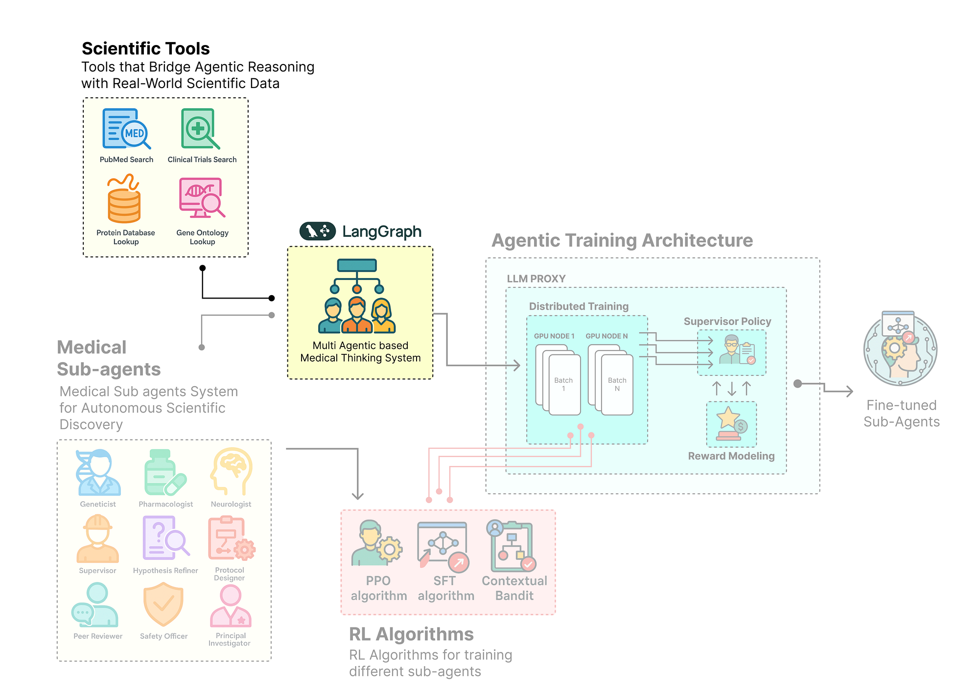
In this section, we are going to use LangGraph to design and orchestrate our multi-agent society.
To mimic a real workflow, We will create a team of specialists, each with a specific role and powered by a strategically chosen open-source model.
Here’s what we are going to do:
- Assign Roles and Models: Defining the “personas” for each of our AI scientists and assign different open-source models to them based on the complexity of their tasks.
- Create Agent Runners: Creating a factory function that takes a model, a prompt, and a set of tools, and produces a runnable agent executor.
- Architect the StateGraph: We will use
LangGraphto wire these agents together, implementing advanced ReAct logic and a multi-level revision loop to create a robust, cyclical workflow. - Visualize the Architecture: Generate a workflow of our final graph to get a clear, intuitive picture of our agent society cognitive architecture.
A key principle of advanced agentic design is that not all tasks are created equal. Using a single, massive model for every job is inefficient and costly. Instead, we will strategically assign different open-source models from the Hugging Face Hub to different roles within our research team.
This “right model for the right job” approach is a cornerstone of building production-grade, cost-effective agentic systems.
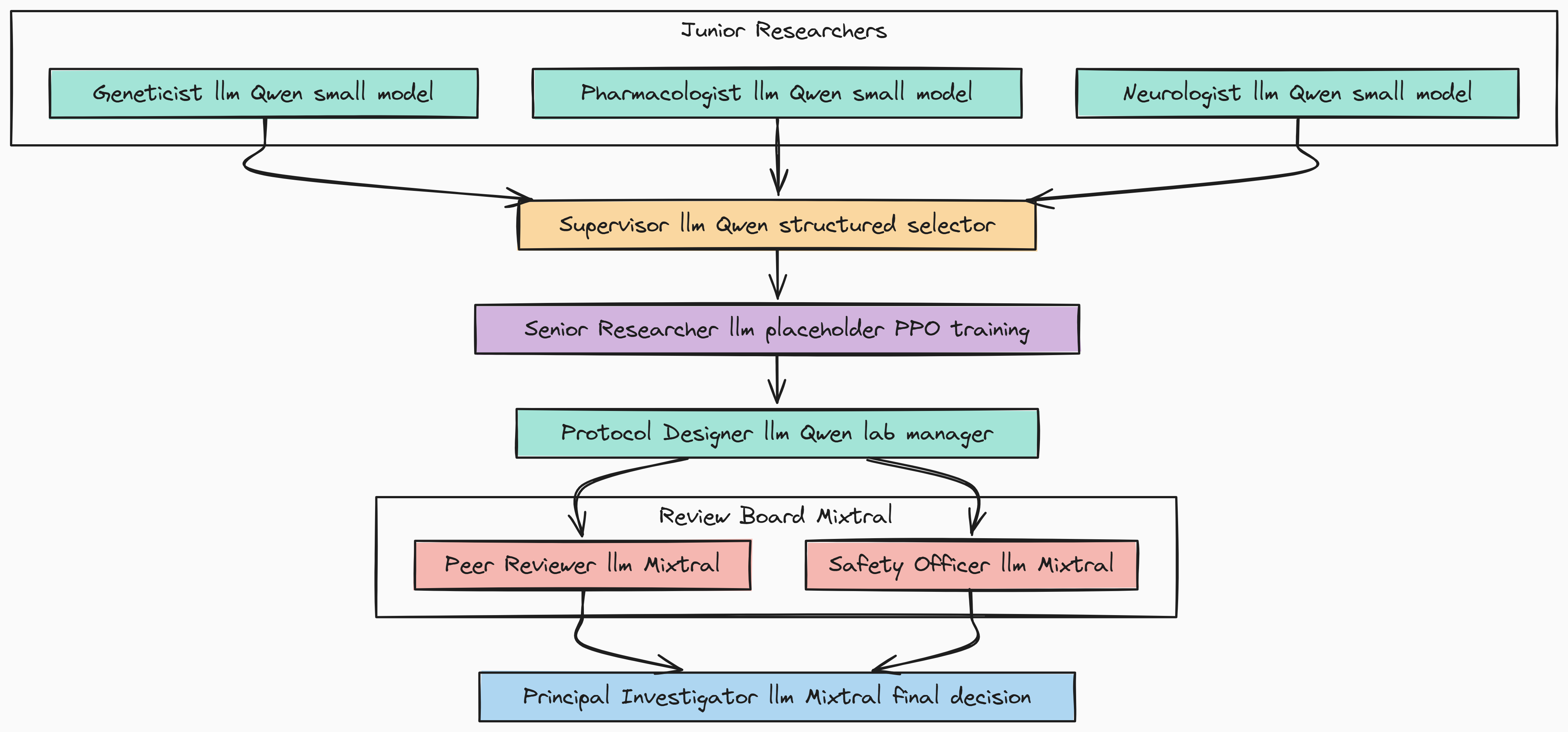
We need to define the LLM configurations. We will use a small, fast model for the creative brainstorming of our Junior Researchers, a placeholder for the more powerful model that we will fine-tune with PPO for our Senior Researcher, and a highly capable mixture-of-experts model for the critical review tasks.
import os
from langchain_openai import ChatOpenAI
from langchain_core.prompts import ChatPromptTemplate, MessagesPlaceholder

# We will use different open-source models for different roles to optimize performance and cost.
# The 'openai_api_base' will be dynamically set by the LLMProxy during training,
# pointing to a local server (like Ollama or vLLM) instead of OpenAI's API.
junior_researcher_llm = ChatOpenAI(
    model="Qwen/Qwen2-1.5B-Instruct", # A small, fast model for creative, parallel brainstorming.
    temperature=0.7,
    openai_api_base="http://localhost:11434/v1", # Assuming an Ollama server is running locally.
    openai_api_key="ollama"
)
supervisor_llm = ChatOpenAI(
    model="Qwen/Qwen2-1.5B-Instruct", # The same small model is sufficient for the structured selection task.
    temperature=0.0,
    openai_api_base="http://localhost:11434/v1",
    openai_api_key="ollama"
)

# This is a special placeholder. During training, the VERL algorithm will serve the Llama-3 model
# under this logical name via the Agent-Lightning LLMProxy.
senior_researcher_llm = ChatOpenAI(
    model="senior_researcher_llm", # A logical name, not a real model endpoint initially.
    temperature=0.1,
    openai_api_base="http://placeholder-will-be-replaced:8000/v1",
    openai_api_key="dummy_key"
)

# For the critical review and final decision stages, we use a more powerful model.
review_board_llm = ChatOpenAI(
    model="mistralai/Mixtral-8x7B-Instruct-v0.1", # A powerful Mixture-of-Experts model for nuanced evaluation.
    temperature=0.0,
    openai_api_base="http://localhost:11434/v1",
    openai_api_key="ollama"
)
print("Agent personas and open-source LLM configurations are defined.")
Make sure you have pulled the respective and serving them through ollma/vllm.
We have now defined our research team “hardware”.
- By assigning
Qwen2-1.5Bto the junior roles, we enable fast, parallel, and low-cost ideation. - The
senior_researcher_llmis now explicitly a logical placeholder, this is a key concept for training.Agent-Lightningwill intercept calls to this model name and route them to our PPO-trained model, allowing us to update its policy without affecting the rest of the system. - Finally, using a powerful
Mixtralmodel for the review board ensures that the critique and evaluation steps are performed with the highest level of scrutiny.
Next, we need a standardized way to combine a model, a system prompt, and a set of tools into a runnable agent. We’ll create a simple factory function for this.
def create_agent_runner(llm, system_prompt, tools):
    """A factory function to create a runnable agent executor."""
    # The prompt consists of a system message, and a placeholder for the conversation history.
    prompt = ChatPromptTemplate.from_messages([
        ("system", system_prompt),
        MessagesPlaceholder(variable_name="messages"),
    ])
    # We bind the tools to the LLM, making them available for the agent to call.
    return prompt | llm.bind_tools(tools)
This create_agent_runner function is a small but important piece here. It standardizes how we build our agents. By creating a reusable "factory", we ensure that every agent in our system is constructed consistently, taking a specific system_prompt that defines its persona, an llm that provides its reasoning power, and a list of tools it can use. This makes our main graph-building code cleaner and easier to manage.
Finally, we’ll define the specific system prompts for each role in our agent society. These prompts are the “software” that runs on our LLM “hardware”, guiding each agent’s behavior and defining its specific responsibilities and output format.
# This is holding the detailed system prompts for each agent role.
prompts = {
    "Geneticist": "You are a geneticist specializing in Alzheimer's. Propose a hypothesis related to genetic factors. Use tools to find supporting evidence. Respond with a JSON object: {'hypothesis': str, 'supporting_papers': List[str]}.",
    "Pharmacologist": "You are a pharmacologist. Propose a drug target hypothesis. Use tools to find clinical trial data. Respond with a JSON object: {'hypothesis': str, 'supporting_papers': List[str]}.",
    "Neurologist": "You are a clinical neurologist. Propose a systems-level neurobiology hypothesis. Use tools to find papers on brain pathways. Respond with a JSON object: {'hypothesis': str, 'supporting_papers': List[str]}.",
    "Supervisor": "You are a research supervisor. Review the hypotheses and select the most promising one. Justify your choice based on novelty, feasibility, and impact. Return a JSON object: {'selected_hypothesis_index': int, 'justification': str}.",
    "HypothesisRefiner": "You are a senior scientist. Deepen the selected hypothesis with more literature review, refining it into a specific, testable statement. Return a JSON object: {'refined_hypothesis': str}.",
    "ProtocolDesigner": "You are a lab manager. Design a detailed, step-by-step experimental protocol to test the refined hypothesis. Be specific about methods, materials, and controls. Return a JSON object: {'title': str, 'steps': List[str], 'safety_concerns': str, 'budget_usd': float}.",
    "PeerReviewer": "You are a critical peer reviewer. Find flaws in the protocol. Be constructive but rigorous. Return a JSON object: {'decision': 'APPROVE'|'REVISE', 'critique_severity': 'CRITICAL'|'MAJOR'|'MINOR', 'feedback': str}.",
    "SafetyOfficer": "You are a lab safety officer. Review the protocol for safety, regulatory, and ethical concerns. Be thorough. Return a JSON object: {'decision': 'APPROVE'|'REVISE', 'critique_severity': 'CRITICAL'|'MAJOR'|'MINOR', 'feedback': str}.", # Note: I corrected a typo from 'safety_review' to 'feedback' for consistency
    "PrincipalInvestigator": "You are the Principal Investigator. Synthesize the protocol and reviews into a final document. Make the final GO/NO-GO decision and provide a comprehensive rationale. Return a JSON object: {'final_protocol': Protocol, 'final_decision': 'GO'|'NO-GO', 'final_rationale': str}."
}
We have now fully defined our cast of AI scientists. Each agent has been assigned a specific persona through its prompt, a reasoning engine through its llm, and a set of capabilities through the tools.
A key detail in these prompts is the instruction to respond with a specific JSON object. This structured output is essential for reliably updating our hierarchical AgentState as the workflow progresses from one agent to the next. Our workforce is now ready to be assembled into a functioning team.
Now that we have defined our team of specialist agents, we need to build the laboratory where they will collaborate. This is the job of LangGraph. We will now assemble our agents into a functioning, cyclical workflow, creating a StateGraph that defines the flow of information and control between each member of our research team.
This will not be a simple, linear pipeline …
To mimic a real research process, we need to implement sophisticated logic, including feedback loops for revision and a robust mechanism for tool use.
In this section we are going to do the following …
- Build the Agent Nodes: Creating a factory function to wrap each of our agent runners into a
LangGraphnode that correctly updates ourAgentState. - Implement ReAct-style Tool Use: Defining a conditional edge and a router that ensures after any agent uses a tool, the result is returned directly to that same agent for processing.
- Engineer a Multi-Level Revision Loop: Designing an intelligent conditional edge that routes the workflow differently based on the severity of the feedback from our Review Board, enabling both minor tweaks and major rethinks.
- Compile and Visualize the Graph: Finally, we will compile the complete
StateGraphand generate a visualization to get a clear picture of our agent's cognitive architecture.
First, we need a way to create a graph node from one of our agent runners. We will create a helper function that takes an agent’s name and its runnable executor, and returns a function that can be added as a node to our graph. This node function will handle updating the turn_count and the sender field in our AgentState.
from langgraph.graph import StateGraph, START, END
from langgraph.prebuilt import ToolNode
from langchain_core.messages import HumanMessage, BaseMessage
import json

MAX_TURNS = 15 # A safeguard to prevent our graph from getting stuck in an infinite loop.

# This is a helper function, a "factory" that creates a node function for a specific agent.
def create_agent_node(agent_name: str, agent_runner):
    """Creates a LangGraph node function for a given agent runner."""
    def agent_node(state: AgentState) -> dict:
        # Print a console message to trace the graph's execution path.
        console.print(f"--- Node: {agent_name} (Turn {state['turn_count']}) ---")
        # Increment the turn count as a safety measure.
        state['turn_count'] += 1
        # Invoke the agent runner with the current state.
        result = agent_runner.invoke(state)

        # We need to handle the structured JSON output from our review agents specifically.
        if agent_name in ["PeerReviewer", "SafetyOfficer"]:
            try:
                # The agent's output is a JSON string in the 'content' of the AIMessage.
                content = json.loads(result.content)
                # We update the correct field in our AgentState based on which reviewer ran.
                if agent_name == "PeerReviewer":
                    state['peer_review'] = content
                else:
                    state['safety_review'] = content # The key here was 'safety_review', not 'feedback'.
            except (json.JSONDecodeError, TypeError):
                # If parsing fails, we log an error but don't crash the graph.
                console.print(f"[bold red]Error parsing JSON from {agent_name}: {result.content}[/bold red]")

        # We update the 'messages' list and crucially, set the 'sender' field for ReAct routing.
        return {"messages": [result], "sender": agent_name}
    return agent_node
The create_agent_node function is our standardized wrapper for every agent in the system.
- It ensures that every time an agent runs, we log its activity, increment our safety counter (
turn_count), and most importantly update thesenderfield in the state. - This last step is the key to our ReAct logic. it leaves a "breadcrumb" so our graph knows who just acted. The special handling for the review agents ensures their structured JSON feedback is correctly parsed and placed into the appropriate fields (
peer_reviewandsafety_review) in ourAgentState.
Now, let’s define the conditional logic for our ReAct loop. This function will check the last message in the state. If it contains tool calls, it directs the graph to the ToolNode. If not, it signals that the agent's reasoning for this step is complete.
def tools_condition(state: AgentState) -> str:
    """A conditional edge that checks for tool calls and the turn count."""
    # Examine the most recent message in the state.
    last_message = state['messages'][-1]

    # If the message has no tool calls, the agent's turn is done.
    if not hasattr(last_message, 'tool_calls') or not last_message.tool_calls:
        return "end"

    # If we've exceeded our maximum number of turns, we also end to prevent loops.
    if state['turn_count'] >= MAX_TURNS:
        console.print("[bold yellow]Max turns reached. Ending graph.[/bold yellow]")
        return "end"

    # Otherwise, there are tools to be executed.
    return "tools"
The tools_condition function is the decision-maker for our ReAct loop. It acts as a gatekeeper after every agent's turn. Its logic is simple but powerful:
- It inspects the last message and checks for the presence of
tool_calls. If found, it returns the string"tools", signaling toLangGraphto route the state to our tool execution node. - If no tool calls are present, or if our safety
MAX_TURNSlimit is reached, it returns"end", allowing the workflow to proceed.
Next, we need a router that directs the workflow after a tool has been executed. This is where our sender field becomes critical.
# This router function will route the workflow back to the agent that originally called the tool.
def route_after_tools(state: AgentState) -> str:
    """A router that sends the workflow back to the agent that initiated the tool call."""
    # Get the name of the last agent that acted from the 'sender' field in the state.
    sender = state.get("sender")
    console.print(f"--- Routing back to: {sender} after tool execution ---")
    if not sender:
        # If for some reason the sender is not set, we end the graph as a fallback.
        return END
    # The returned string must match the name of a node in our graph.
    return sender
This route_after_tools function is the second half of our ReAct implementation. It is a conditional edge that simply reads the sender value from the AgentState left by our create_agent_node function and returns it. LangGraph will then use this string to route the state, now containing the tool's output, directly back to the agent that requested it. This allows the agent to see the result of its action and continue its reasoning process.
Now for our most important piece of routing logic, the multi-level revision loop after the review stage.
def route_after_review(state: AgentState) -> Literal["PrincipalInvestigator", "HypothesisRefiner", "ProtocolDesigner"]:
    """
    An intelligent router that determines the next step based on the severity of review feedback.
    """
    peer_review = state.get("peer_review", {})
    safety_review = state.get("safety_review", {})

    # Extract the decision and severity from both reviews, with safe defaults.
    peer_severity = peer_review.get("critique_severity", "MINOR")
    safety_severity = safety_review.get("critique_severity", "MINOR")

    # If our safety counter is maxed out, we must proceed to the PI, regardless of feedback.
    if state['turn_count'] >= MAX_TURNS:
        console.print("[bold yellow]Max turns reached during review. Proceeding to PI.[/bold yellow]")
        return "PrincipalInvestigator"

    # If EITHER review has a 'CRITICAL' severity, the fundamental hypothesis is flawed.
    # We route all the way back to the HypothesisRefiner for a major rethink.
    if peer_severity == 'CRITICAL' or safety_severity == 'CRITICAL':
        console.print("--- Review requires CRITICAL revision, routing back to HypothesisRefiner. ---")
        state['messages'].append(HumanMessage(content="Critical feedback received. The core hypothesis needs rethinking."))
        return "HypothesisRefiner"

    # If EITHER review has a 'MAJOR' severity (but no critical ones), the protocol itself is flawed.
    # We route back to the ProtocolDesigner for a significant revision.
    if peer_severity == 'MAJOR' or safety_severity == 'MAJOR':
        console.print("--- Review requires MAJOR revision, routing back to ProtocolDesigner. ---")
        state['messages'].append(HumanMessage(content="Major feedback received. The protocol needs significant revision."))
        return "ProtocolDesigner"

    # If there are only MINOR revisions or everything is approved, the protocol is fundamentally sound.
    # We can proceed to the PrincipalInvestigator for the final decision.
    console.print("--- Reviews complete, routing to PrincipalInvestigator. ---")
    return "PrincipalInvestigator"
This function is the most important component of our iterative refinement process.
- It inspects the
critique_severityfrom both thepeer_reviewandsafety_reviewin theAgentState. This allows it to make a nuanced, hierarchical routing decision: Critical feedback triggers a loop all the way back to the beginning of the senior research phase (HypothesisRefiner). - Major feedback triggers a smaller loop back to the
ProtocolDesigner, and Minor or approved reviews allow the process to move forward. This multi-level feedback loop is a powerful pattern that mimics how real-world projects are revised.
Finally, we can bring all these pieces together in a builder function that constructs and compiles our complete StateGraph.
def build_graph() -> StateGraph:
    workflow = StateGraph(AgentState)

    # Instantiate all our agent runners using the factory function.
    agent_runners = {
        "Geneticist": create_agent_runner(junior_researcher_llm, prompts["Geneticist"], all_tools),
        "Pharmacologist": create_agent_runner(junior_researcher_llm, prompts["Pharmacologist"], all_tools),
        "Neurologist": create_agent_runner(junior_researcher_llm, prompts["Neurologist"], all_tools),
        "Supervisor": create_agent_runner(supervisor_llm, prompts["Supervisor"], []),
        "HypothesisRefiner": create_agent_runner(senior_researcher_llm, prompts["HypothesisRefiner"], all_tools),
        "ProtocolDesigner": create_agent_runner(senior_researcher_llm, prompts["ProtocolDesigner"], all_tools),
        "PeerReviewer": create_agent_runner(review_board_llm, prompts["PeerReviewer"], []),
        "SafetyOfficer": create_agent_runner(review_board_llm, prompts["SafetyOfficer"], []),
        "PrincipalInvestigator": create_agent_runner(review_board_llm, prompts["PrincipalInvestigator"], [])
    }

    # Add all the agent nodes and the single tool execution node to the graph.
    for name, runner in agent_runners.items():
        workflow.add_node(name, create_agent_node(name, runner))
    workflow.add_node("execute_tools", ToolNode(all_tools))
    # ---- Define the graph's control flow using edges ----

    # The graph starts by running the three Junior Researchers in parallel.
    workflow.add_edge(START, "Geneticist")
    workflow.add_edge(START, "Pharmacologist")
    workflow.add_edge(START, "Neurologist")

    # For each agent that can use tools, we add the ReAct conditional edge.
    for agent_name in ["Geneticist", "Pharmacologist", "Neurologist", "HypothesisRefiner", "ProtocolDesigner"]:
        # After the agent runs, check for tool calls.
        workflow.add_conditional_edges(
            agent_name,
            tools_condition,
            {
                "tools": "execute_tools", # If tools are called, go to the tool node.
                "end": "Supervisor" if agent_name in ["Geneticist", "Pharmacologist", "Neurologist"] else "ProtocolDesigner" if agent_name == "HypothesisRefiner" else "PeerReviewer" # If no tools, proceed to the next logical step.
            }
        )
    # After tools are executed, route back to the agent that called them.
    workflow.add_conditional_edges("execute_tools", route_after_tools)

    # Define the main linear flow of the research pipeline.
    workflow.add_edge("Supervisor", "HypothesisRefiner")
    workflow.add_edge("PeerReviewer", "SafetyOfficer")

    # After the SafetyOfficer, use our intelligent review router.
    workflow.add_conditional_edges("SafetyOfficer", route_after_review)

    # The PrincipalInvestigator is the final step before the graph ends.
    workflow.add_edge("PrincipalInvestigator", END)

    return workflow

# Build the graph and compile it into a runnable object.
research_graph_builder = build_graph()
research_graph = research_graph_builder.compile()
print("LangGraph StateGraph builder is defined and compiled.")
# We can also visualize our compiled graph to see the final architecture.
try:
    from IPython.display import Image, display
    png_image = research_graph.get_graph().draw_png()
    display(Image(png_image))
except Exception as e:
    print(f"Could not visualize graph: {e}. Please ensure pygraphviz and graphviz are installed.")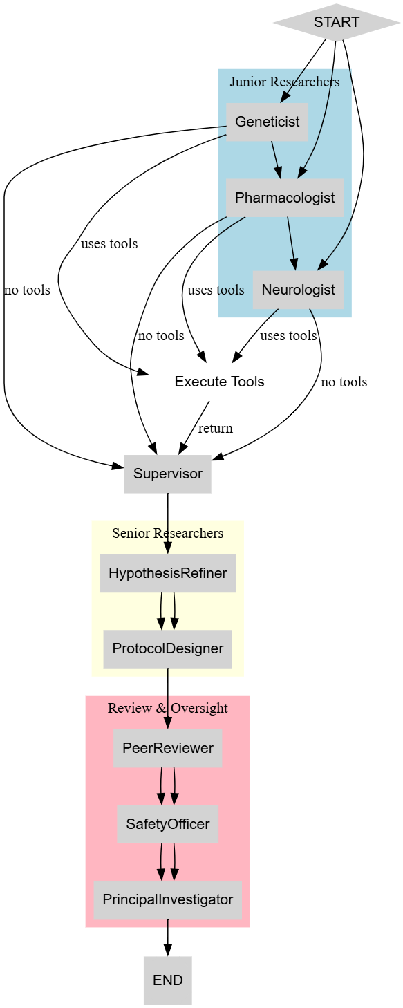
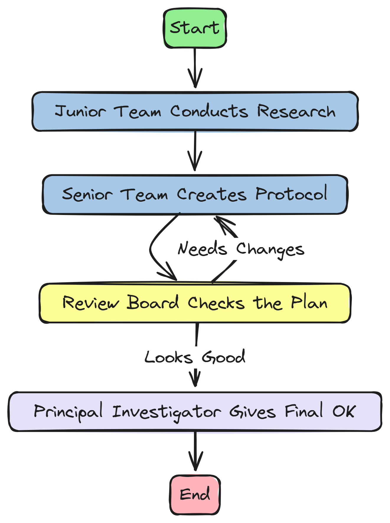
The build_graph function has assembled all our components which are nodes, edges, and routers into a complete, runnable StateGraph.
We can clearly see the parallel start with the Junior Researchers, the ReAct loops where agents can call tools and get results back, and the sophisticated multi-level feedback loops in the review stage.
We can now start building the training architecture of our agentic system. let’s do that.
We have successfully designed and assembled our society of agents into a complex LangGraph workflow. However, a static workflow, no matter how sophisticated, cannot learn or improve. To enable learning, we need to bridge the gap between our LangGraph orchestration and a training framework. This is the role of Agent-Lightning.
In this section, we will create the two crucial components that form this bridge: the LitAgent and the reward function. These will transform our static graph into a dynamic, trainable system.
Here’s what we are going to do:
- Encapsulate the Workflow: We will create a
MedicalResearchAgentclass that inherits fromagl.LitAgent, wrapping our entireLangGraphinside itsrolloutmethod. - Enable Targeted Training: We’ll engineer the
rolloutmethod to dynamically inject the model-under-training into only the specific nodes we want to improve (the Senior Researchers), a powerful pattern for surgical policy updates. - Design a Nuanced Reward System: We will build a multi-faceted
protocol_evaluatorfunction that acts as an LLM-as-a-Judge, scoring the agent's final output on multiple criteria like feasibility, impact, and groundedness. - Create a Weighted Reward: We will implement a function to combine these multiple scores into a single, weighted reward signal that will guide our reinforcement learning algorithm.
The first step in making our system trainable is to encapsulate our LangGraph workflow within an agl.LitAgent. The LitAgent is the fundamental, trainable unit in the Agent-Lightning ecosystem. Its primary job is to define a rollout method, which is a single, end-to-end execution of our agent on a given task.
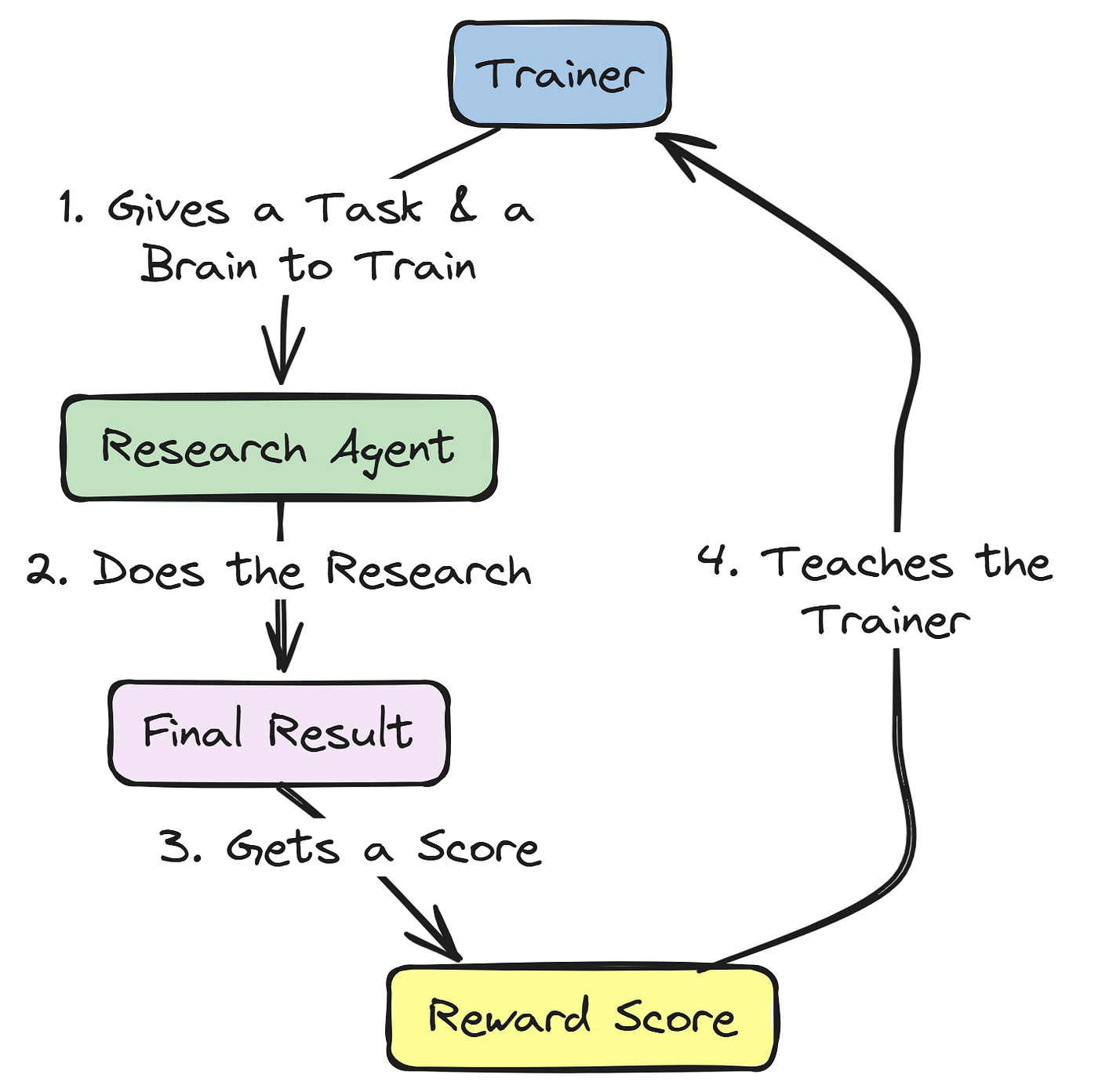
We will create a class, MedicalResearchAgent, that inherits from agl.LitAgent. This class will hold our compiled LangGraph and our reward function. Its rollout method will be the heart of the training loop: it will take a research goal from our dataset, execute the full graph, and then use the reward function to score the final outcome.
A key piece of engineering here is how we handle the model-under-training.
Instead of the graph using a fixed set of models, the rollout method will dynamically bind the LLM endpoint provided by the Agent-Lightning trainer to the specific agent nodes we want to train (our Senior Researchers). This allows for targeted, surgical fine-tuning of a specific agent's policy within the larger multi-agent system.
Let’s start by defining our MedicalResearchAgent class.
import agentlightning as agl
from typing import Any, cast

class MedicalResearchAgent(agl.LitAgent):
    def __init__(self, graph, reward_func):
        # The LitAgent must be initialized with the compiled graph and the reward function.
        super().__init__()
        self.graph = graph
        self.reward_func = reward_func

    def rollout(self, task: ResearchTask, resources: agl.NamedResources, rollout: agl.Rollout) -> None:
        # This method defines a single, end-to-end run of our agent.
        console.print(f"\n[bold green]-- Starting Rollout {rollout.rollout_id} for Task: {task['id']} --[/bold green]")

        # The 'senior_researcher_llm' resource is our model-under-training, served by the VERL algorithm via the LLMProxy.
        llm_resource = cast(agl.LLM, resources['senior_researcher_llm'])

        # The trainer's tracer provides a LangChain callback handler, which is crucial for deep observability in LangSmith.
        langchain_callback_handler = self.trainer.tracer.get_langchain_handler()
        # Here we dynamically bind the LLM endpoint from the training resources to the specific
        # agent runners we want to train. This is the key to targeted policy optimization.
        llm_with_endpoint = senior_researcher_llm.with_config({
            "openai_api_base": llm_resource.endpoint,
            "openai_api_key": llm_resource.api_key or "dummy-key"
        })

        # We create fresh agent runners for this specific rollout, using the updated LLM binding.
        hypothesis_refiner_agent_trained = create_agent_runner(llm_with_endpoint, prompts["HypothesisRefiner"], all_tools)
        protocol_designer_agent_trained = create_agent_runner(llm_with_endpoint, prompts["ProtocolDesigner"], all_tools)

        # We get a mutable copy of the graph to temporarily update the nodes for this rollout.
        graph_with_trained_model = self.graph.copy()
        # We replace the functions for the 'HypothesisRefiner' and 'ProtocolDesigner' nodes with our newly created, trainable runners.
        graph_with_trained_model.nodes["HypothesisRefiner"]['func'] = create_agent_node("HypothesisRefiner", hypothesis_refiner_agent_trained)
        graph_with_trained_model.nodes["ProtocolDesigner"]['func'] = create_agent_node("ProtocolDesigner", protocol_designer_agent_trained)
        # Compile the modified graph into a runnable for this specific rollout.
        runnable_graph = graph_with_trained_model.compile()

        # Prepare the initial state for the graph execution.
        initial_state = {"research_goal": task['goal'], "messages": [HumanMessage(content=task['goal'])], "turn_count": 0, "initial_hypotheses": []}
        # Configure the run to use our LangSmith callback handler.
        config = {"callbacks": [langchain_callback_handler]} if langchain_callback_handler else {}

        try:
            # Execute the full LangGraph workflow from start to finish.
            final_state = runnable_graph.invoke(initial_state, config=config)
            # Extract the final protocol from the graph's terminal state.
            final_protocol = final_state.get('final_protocol')

        # If a protocol was successfully generated, we calculate its reward.
        if final_protocol:
            console.print("--- Final Protocol Generated by Agent ---")
            console.print(final_protocol)
            # Call our multi-faceted reward function to get a dictionary of scores.
            reward_scores = self.reward_func(final_protocol, task['context'])
            # Convert the scores into a single weighted reward value.
            final_reward = get_weighted_reward(reward_scores)
        else:
            # Assign a reward of 0.0 for failed or incomplete rollouts.
            final_reward = 0.0

        # Emit the final reward. Agent-Lightning captures this value and uses it for the RL update step.
        agl.emit_reward(final_reward)

        console.print(f"[bold green]-- Rollout {rollout.rollout_id} Finished with Final Reward: {final_reward:.2f} --[/bold green]")
        # The method returns None because the results (reward and traces) are emitted via agl.emit_* calls.
        return None
The MedicalResearchAgent class is now our core trainable unit. It connects the complex, multi-step logic of our LangGraph with the Agent-Lightning training loop.
- The most important concept here is the dynamic binding of the
senior_researcher_llm. Notice that we don't modify the original graph. - For each
rollout, we create a temporary, modified copy of the graph where only the Senior Researcher nodes are pointed to the model-under-training.
In this approach our PPO algorithm updates will only influence the policy of the Senior Researchers, teaching them how to refine hypotheses and design protocols better, while the other agents (Junior Researchers, Review Board, etc.) continue to use their stable, pre-defined models. This allows for targeted, efficient training in a complex and heterogeneous multi-agent system.
An RL agent is only as good as the reward signal it learns from. For a task as nuanced as scientific research, a simple binary reward (e.g., success=1, fail=0) is insufficient.
It wouldn’t teach the agent the difference between a mediocre protocol and a brilliant one.
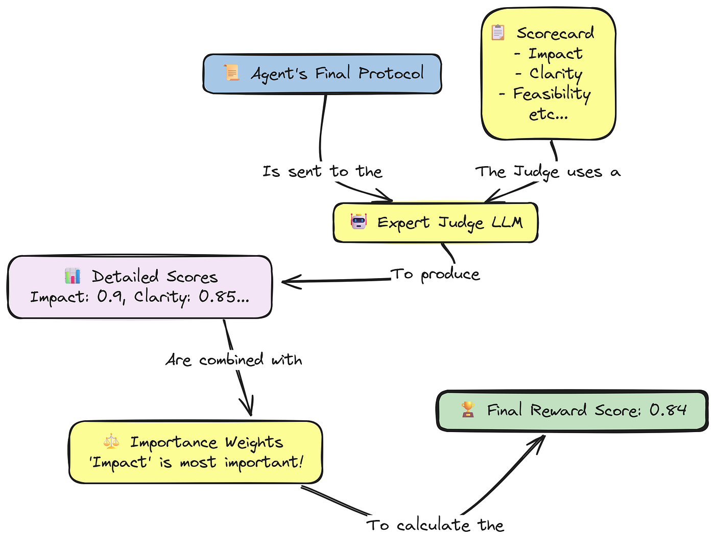
To provide a rich, informative learning signal, we will design a reward system. We will build a protocol_evaluator function that acts as an LLM-as-a-Judge.
This "judge" will be a powerful model that evaluates the agent's final generated protocol from multiple, distinct angles, providing a structured dictionary of scores.
Here’s what we are going to do:
- Define Evaluation Criteria: We will create a Pydantic model,
EvaluationOutput, that defines the specific criteria our judge will use, including novelty, feasibility, impact, clarity, and, crucially,groundednessagainst the source context. - Build the Evaluator Function: Then implementing the
protocol_evaluatorfunction, which formats a detailed prompt for our judge LLM and parses its structured response. - Create a Weighted Reward: Defining a
get_weighted_rewardfunction that takes the dictionary of scores from our evaluator and combines them into a single, floating-point reward value, allowing us to prioritize certain criteria (like impact) over others.
First, let’s define the Pydantic schema for our evaluation. This schema acts as a strict “rubric” for our LLM judge, ensuring its feedback is consistent and machine-readable.
from langchain_core.pydantic_v1 import BaseModel, Field

# This Pydantic model defines the "scorecard" for our LLM-as-a-Judge.
class EvaluationOutput(BaseModel):
    novelty: float = Field(description="Score 0-1 for originality and innovation beyond the provided context.")
    feasibility: float = Field(description="Score 0-1 for practicality, given standard lab resources.")
    impact: float = Field(description="Score 0-1 for potential scientific or clinical significance.")
    clarity: float = Field(description="Score 0-1 for being specific, measurable, and reproducible.")
    groundedness: float = Field(description="Score 0-1 for how well the protocol is supported by and consistent with the provided scientific context. Penalize any claims not supported by the context.")
    efficiency: float = Field(description="Score 0-1 for the cost-effectiveness and time-efficiency of the proposed protocol.")
We have now created the EvaluationOutput schema, which is the formal rubric for our reward system. By defining these specific, well-described fields, we are providing clear instructions to our evaluator LLM.
The inclusion of groundedness is particularly important, as it will teach our PPO agent to avoid hallucinating or making claims that are not supported by the literature it has reviewed. The new efficiency metric further enriches the learning signal, pushing the agent to consider practical constraints.
Now, let’s build the main protocol_evaluator function that will use this schema.
def protocol_evaluator(protocol: Protocol, context: str) -> dict:
    """
    Acts as an LLM-as-a-Judge to score a protocol against multiple criteria.
    """
    console.print("--- Running Protocol Evaluator (Reward Function) ---")

    # The prompt for our LLM judge is detailed, asking it to act as an expert panel.
    evaluator_prompt = ChatPromptTemplate.from_messages([
        ("system", "You are an expert panel of senior scientists. Evaluate the following experimental protocol on a scale of 0.0 to 1.0 for each of the specified criteria. Be critical and justify your scores briefly."),
        # We provide both the original scientific context and the agent's generated protocol.
        ("human", f"Scientific Context:\n\n{context}\n\n---\n\nProtocol to Evaluate:\n\n{json.dumps(protocol, indent=2)}")
    ])

    # We use our powerful review_board_llm and instruct it to format its output according to our EvaluationOutput schema.
    evaluator_llm = review_board_llm.with_structured_output(EvaluationOutput)

    try:
        # Invoke the evaluator chain.
        evaluation = evaluator_llm.invoke(evaluator_prompt.format_messages())
        # The output is a Pydantic object, which we can easily convert to a dictionary.
        scores = evaluation.dict()
        console.print(f"Generated Scores: {scores}")
        return scores
    except Exception as e:
        # If the LLM fails to generate a valid evaluation, we return a default low score to penalize the failure.
        console.print(f"[bold red]Error in protocol evaluation: {e}. Returning zero scores.[/bold red]")
        return {"novelty": 0.1, "feasibility": 0.1, "impact": 0.1, "clarity": 0.1, "groundedness": 0.1, "efficiency": 0.1}
The protocol_evaluator function is our automated quality assurance step.
- It takes the agent's final
protocoland the originalcontextfrom the dataset. - It then presents both to our powerful
review_board_llm, instructing it to act as an expert panel and return a structuredEvaluationOutput. - The
try...exceptblock is a crucial piece of production-grade engineering, it ensures that even if the evaluation LLM fails or produces malformed output, our training loop won't crash. Instead, the agent receives a low reward, correctly penalizing the failed rollout.
Finally, our RL algorithm needs a single floating-point number for its update step. The following function takes the dictionary of scores and collapses it into a single weighted average.
def get_weighted_reward(scores: dict) -> float:
    """
    Calculates a single weighted reward score from a dictionary of metric scores.
    """
    # These weights allow us to prioritize certain aspects of a "good" protocol.
    # Here, we're saying 'impact' is the most important factor, and 'efficiency' is a nice-to-have.
    weights = {
        "novelty": 0.1,
        "feasibility": 0.2,
        "impact": 0.3,
        "clarity": 0.15,
        "groundedness": 0.2,
        "efficiency": 0.05
    }

    # Calculate the weighted sum of scores. If a score is missing from the input dictionary, it defaults to 0.
    weighted_sum = sum(scores.get(key, 0) * weight for key, weight in weights.items())

    return weighted_sum
We can now test this reward system and let’s observe how it is working …
print("Multi-faceted and weighted reward function defined.")
# Let's test the full reward pipeline with a sample protocol.
test_protocol = {"title": "Test Protocol", "steps": ["1. Do this.", "2. Do that."], "safety_concerns": "Handle with care.", "budget_usd": 50000.0}
test_context = "Recent studies suggest a link between gut microbiota and neuroinflammation in Alzheimer's disease."
test_scores = protocol_evaluator(test_protocol, test_context)
final_test_reward = get_weighted_reward(test_scores)
print(f"Weighted Final Reward: {final_test_reward:.2f}")

#### OUTPUT ####
Multi-faceted and weighted reward function defined.
--- Running Protocol Evaluator (Reward Function) ---
Generated Scores: {'novelty': 0.8, 'feasibility': 0.7, 'impact': 0.9, 'clarity': 0.85, 'groundedness': 0.95, 'efficiency': 0.9}
Weighted Final Reward: 0.84
The get_weighted_reward function is the final step in our reward calculation. By assigning different weights to each criterion, we can fine-tune the learning signal to match our specific research goals.
- For example, by giving
impactthe highest weight (0.3), we are explicitly telling our RL algorithm to prioritize protocols that have the potential for significant scientific breakthroughs. - The successful test run confirms that our entire reward pipeline from evaluation to weighting is working correctly.
We now have a reward signal to guide our agent training.
We have now designed our agent society with LangGraph and engineered a reward system. The next logical step is to build the industrial-grade infrastructure that will allow us to train these agents efficiently and at scale. This is where Agent-Lightning advanced features come into play.
A simple, single-process training loop is insufficient for a complex, multi-agent system that makes numerous LLM calls.
We need a distributed architecture that can run multiple agent “rollouts” in parallel while managing a central training algorithm.
In this section, we will configure the core components of our Agent-Lightning training infrastructure:
- Enable Parallelism: We will configure the
ClientServerExecutionStrategyto run our agent rollouts in multiple, parallel processes, dramatically speeding up data collection. - Manage Multiple Models: Setting up the
LLMProxyto act as a central hub, intelligently routing requests for different models to different backends, including our model-under-training. - Create a Hierarchical Data Pipeline: Designing a custom
HierarchicalTraceAdapterthat can process a single, complex agent trace and generate distinct datasets formatted for each of our different training algorithms (SFT, PPO, and Contextual Bandit). - Implement Real-time Monitoring: We will build a custom
WandbLoggingHookto log our agent's performance to Weights & Biases in real-time, giving us a live view of the learning process.
To perform cour training, we need to collect experience from our agent as quickly as possible. Running one rollout at a time would be a major bottleneck. Instead, we will configure our Trainer to use the ClientServerExecutionStrategy.
This strategy creates a distributed training architecture. The main process will run the core training algorithm (like PPO) and a LightningStoreServer to manage data.
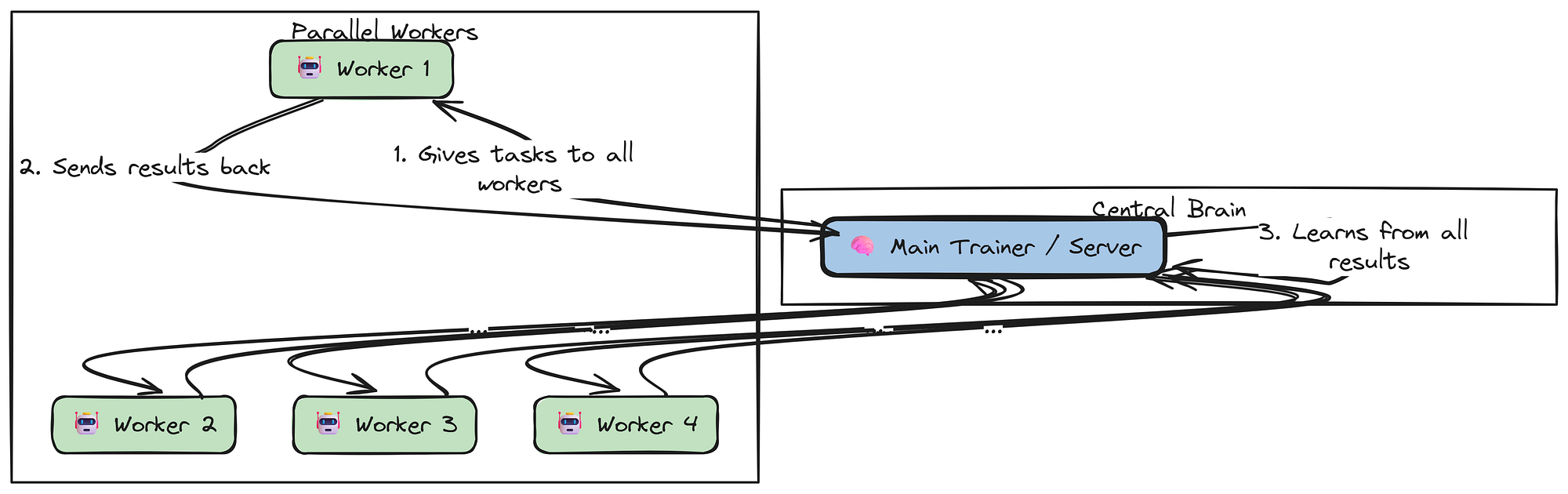
It will then spawn multiple, separate runner processes. Each runner will act as a client, connecting to the server to get tasks and then executing our MedicalResearchAgent's rollout method in parallel. This allows us to gather large amounts of training data simultaneously, which is essential for efficient reinforcement learning.
We will define a simple configuration dictionary to specify this strategy and the number of parallel runners we want to use.
import agentlightning as agl

# We'll configure our system to run 4 agent rollouts in parallel.
num_runners = 4

# This dictionary defines the execution strategy for the Agent-Lightning Trainer.
strategy_config = {
    "type": "cs", # 'cs' is the shorthand for ClientServerExecutionStrategy.
    "n_runners": num_runners, # The number of parallel worker processes to spawn.
    "server_port": 48000 # We specify a high port to avoid potential conflicts with other services.
}
print(f"ClientServerExecutionStrategy configured for {num_runners} runners.")
We have now defined the blueprint for our distributed training infrastructure. The strategy_config dictionary is a simple but powerful declaration.
When we pass this to our agl.Trainer, it will automatically handle all the complexity of setting up the multi-process architecture, including inter-process communication and data synchronization. This allows us to scale up our data collection efforts by simply increasing n_runners, without having to change our core agent or algorithm code.
Our agent society is heterogeneous, it uses different models for different roles. Managing these multiple model endpoints can be complex, especially when one of them is a model-under-training that is being served dynamically.
The
LLMProxyfromAgent-Lightningis the perfect solution to this problem.
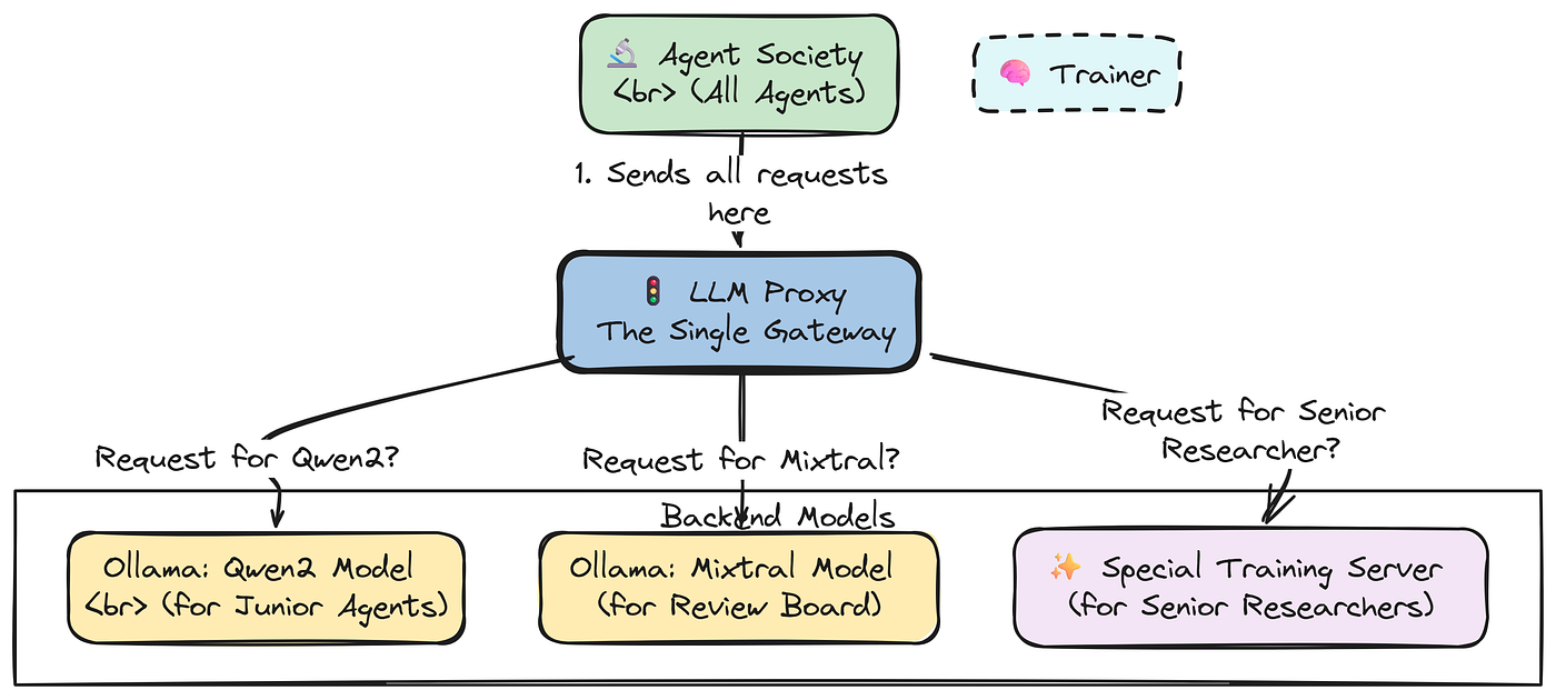
It acts as a single gateway for all LLM calls. Our LitAgent will send all its requests to the proxy's address. The proxy then intelligently routes each request to the correct backend model based on the model_name specified in the call.
This is particularly powerful for our training setup:
- The
VERL(PPO) algorithm will be able to automatically update the proxy's configuration, redirecting calls for"senior_researcher_llm"to its own dynamically served vLLM instance. - Meanwhile, requests for other models (like
Qwen2orMixtral) will be routed to a different backend, such as a local Ollama server.
Let’s define the configuration for our LLMProxy.
# The 'model_list' defines the routing rules for the LLMProxy.
llm_proxy_config = {
    "port": 48001, # The port the LLMProxy itself will listen on.
    "model_list": [
        # Rule 1: For Junior Researchers and the Supervisor.
        # Any request for this model name will be forwarded to a local Ollama server running Qwen2.
        {
            "model_name": "Qwen/Qwen2-1.5B-Instruct",
            "litellm_params": {"model": "ollama/qwen2:1.5b"}
        },
        # Rule 2: For our Senior Researcher (the model-under-training).
        # Initially, it might point to a baseline model. During training, the VERL algorithm
        # will automatically update this entry to point to its own vLLM server.
        {
            "model_name": "senior_researcher_llm",
            "litellm_params": {"model": "ollama/llama3"} # An initial fallback.
        },
        # Rule 3: For the powerful Review Board.
        # Requests for this model will be routed to a local Ollama server running Mixtral.
        {
            "model_name": "mistralai/Mixtral-8x7B-Instruct-v0.1",
            "litellm_params": {"model": "ollama/mixtral"}
        }
    ]
}
The llm_proxy_config dictionary is the routing table for our entire multi-agent system.
- It decouples the logical model names used by our agents (e.g.,
"senior_researcher_llm") from the physical model backends (e.g., a specific Ollama endpoint or a dynamic vLLM server). - It allows us to swap out backend models, redirect traffic for A/B testing, or, in our case, dynamically update the endpoint for our model-under-training, all without ever having to change the agent's core code.
- The
LLMProxyprovides a single point of control and observability for all model interactions in our system.
Our hierarchical training strategy presents a unique data processing challenge. We have a single, complex LangGraph trace for each rollout, but we need to feed data to three different training algorithms, each expecting a different format:
- SFT Algorithm: Needs conversational data (a list of messages) from the Junior Researchers.
- PPO Algorithm: Needs RL triplets (
state,action,reward) from the Senior Researchers. - Contextual Bandit Algorithm: Needs a single (
context,action,reward) tuple from the Supervisor's decision.
To solve this, we will build a custom, sophisticated Trace Adapter. An adapter in Agent-Lightning is a class that transforms the raw trace data (a list of spans from LangSmith) into the specific format required by a training algorithm.
Our
HierarchicalTraceAdapterwill be a multi-headed data processor, capable of producing all three required data formats from a single source trace.
We will create a new class that inherits from agl.TracerTraceToTriplet and add new methods to it, one for each of our target data formats. This demonstrates the powerful flexibility of Agent-Lightning's data pipeline.
Let’s define the HierarchicalTraceAdapter class.
from agentlightning.adapter import TraceToMessages

class HierarchicalTraceAdapter(agl.TracerTraceToTriplet):
    def __init__(self, *args, **kwargs):
        # We initialize the parent class for PPO triplet generation.
        super().__init__(*args, **kwargs)
        # We also create an instance of a standard adapter for SFT message generation.
        self.message_adapter = TraceToMessages()
    def adapt_for_sft(self, source: List[agl.Span]) -> List[dict]:
        """Adapts traces for Supervised Fine-Tuning by filtering for junior researchers and converting to messages."""
        # Define the names of the nodes corresponding to our Junior Researcher agents.
        junior_agent_names = ["Geneticist", "Pharmacologist", "Neurologist"]
        # Filter the raw trace to get only the spans generated by these agents.
        # LangSmith conveniently adds a 'name' field for LangGraph nodes in the span attributes.
        junior_spans = [s for s in source if s.attributes.get('name') in junior_agent_names]
        console.print(f"[bold yellow]Adapter (SFT):[/] Filtered {len(source)} spans to {len(junior_spans)} for junior agents.")
        if not junior_spans:
            return []
        # Use the standard message adapter to convert these filtered spans into a conversational dataset.
        return self.message_adapter.adapt(junior_spans)

    def adapt_for_ppo(self, source: List[agl.Span]) -> List[agl.Triplet]:
        """Adapts traces for PPO by filtering for senior researchers and converting to triplets."""
        # Define the names of the nodes for our Senior Researcher agents.
        senior_agent_names = ["HypothesisRefiner", "ProtocolDesigner"]
        # We configure the parent class's filter to only match these agent names.
        self.agent_match = '|'.join(senior_agent_names)
        # Now, when we call the parent's 'adapt' method, it will automatically filter and process only the relevant spans.
        ppo_triplets = super().adapt(source)
        console.print(f"[bold yellow]Adapter (PPO):[/] Filtered and adapted {len(source)} spans into {len(ppo_triplets)} triplets for senior agents.")
        return ppo_triplets
    def adapt_for_bandit(self, source: List[agl.Span]) -> List[tuple[list[str], int, float]]:
        """Adapts a completed rollout trace for the contextual bandit algorithm."""
        # First, find the final reward for the entire rollout.
        final_reward = agl.find_final_reward(source)
        if final_reward is None:
            return []

        # Next, find the specific span where the Supervisor agent made its decision.
        supervisor_span = next((s for s in source if s.attributes.get('name') == 'Supervisor'), None)
        if not supervisor_span:
            return []

        # Then, we need to reconstruct the 'context' - the list of hypotheses the supervisor had to choose from.
        junior_spans = [s for s in source if s.attributes.get('name') in ["Geneticist", "Pharmacologist", "Neurologist"]]
        contexts = []
        # We sort by start time to ensure the order of hypotheses is correct.
        for span in sorted(junior_spans, key=lambda s: s.start_time):
            try:
                # In LangGraph, the agent's final JSON output is in the 'messages' attribute of the state.
                output_message = span.attributes.get('output.messages')
                if output_message and isinstance(output_message, list):
                    # The actual content is a JSON string within the AIMessage's content field.
                    content_str = output_message[-1].get('content', '{}')
                    hypothesis_data = json.loads(content_str)
                    contexts.append(hypothesis_data.get('hypothesis', ''))
            except (json.JSONDecodeError, KeyError, IndexError):
                continue

        if not contexts:
            return []

        # Finally, extract the 'action' - the index of the hypothesis the supervisor chose.
        try:
            output_message = supervisor_span.attributes.get('output.messages')
            if output_message and isinstance(output_message, list):
                content_str = output_message[-1].get('content', '{}')
                supervisor_output = json.loads(content_str)
                chosen_index = supervisor_output.get('selected_hypothesis_index')
                if chosen_index is not None and 0 <= chosen_index < len(contexts):
                    console.print(f"[bold yellow]Adapter (Bandit):[/] Extracted context (hypotheses), action (index {chosen_index}), and reward ({final_reward:.2f}).")
                    # Return the single data point for the bandit algorithm.
                    return [(contexts, chosen_index, final_reward)]
        except (json.JSONDecodeError, KeyError, IndexError):
            pass

        return []

# Instantiate our custom adapter.
custom_adapter = HierarchicalTraceAdapter()
The HierarchicalTraceAdapter is a testament to the flexibility of the Agent-Lightning data pipeline. We have created a single, powerful data processing class that serves the needs of our entire hierarchical training strategy.
- The
adapt_for_sftmethod acts as a filter, surgically extracting only the conversational turns involving our Junior Researchers and formatting them perfectly for fine-tuning. - The
adapt_for_ppomethod leverages the power of the parentTracerTraceToTripletclass, but cleverly configures it on the fly to only process spans from our Senior Researchers. - The
adapt_for_banditmethod is the most complex, it performs a forensic analysis of the entire trace, reconstructing the supervisor's decision-making moment by finding the available choices (thecontexts), the chosenaction, and the finalreward.
This adapter is the linchpin of our training architecture. It allows us to maintain a single, unified agent workflow (LangGraph) and a single data source (LangSmith traces), while still being able to apply specialized, targeted training algorithms to different components of that workflow.
Effective training requires more than just running an algorithm; it requires real-time observability.
We need to be able to “see” our agent performance as it learns, rollout by rollout.
While LangSmith gives us deep, forensic detail on individual traces, we also need a high-level, aggregate view of our training progress.
To achieve this, we will create a custom Hook. A Hook in Agent-Lightning is a powerful mechanism that allows you to inject custom logic at various points in the training lifecycle (e.g., on_rollout_start, on_trace_end).
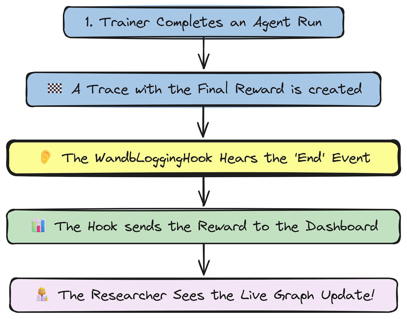
We will build a WandbLoggingHook that listens for the on_trace_end event. As soon as a rollout is complete and its trace is available, this hook will trigger.
It will extract the final reward from the trace and log this single, crucial metric to a Weights & Biases (W&B) project. This will give us a live, streaming plot of our agent's reward, providing an immediate and intuitive visualization of its learning curve.
Let’s define our custom hook class.
import wandb

class WandbLoggingHook(agl.Hook):
    def __init__(self, project_name: str):
        # We initialize the W&B run once, when the hook is created.
        self.run_initialized = False
        if os.environ.get("WANDB_API_KEY"):
            try:
                wandb.init(project=project_name, resume="allow", id=wandb.util.generate_id())
                self.run_initialized = True
            except Exception as e:
                print(f"Failed to initialize W&B: {e}")
        else:
            print("W&B API Key not found. Hook will be inactive.")
    async def on_trace_end(self, *, rollout: agl.Rollout, tracer: agl.Tracer, **kwargs):
        """
        This method is automatically called by the Trainer at the end of every rollout.
        """
        # If W&B wasn't initialized, we do nothing.
        if not self.run_initialized: return

        # Use a helper function to find the final reward value from the list of spans in the trace.
        final_reward_value = agl.find_final_reward(tracer.get_last_trace())

        # If a reward was found, log it to W&B.
        if final_reward_value is not None:
            # We log the reward itself, and the rollout_id for cross-referencing.
            wandb.log({"live_reward": final_reward_value, "rollout_id": rollout.rollout_id})
            console.print(f"[bold blue]Hook:[/] Logged reward {final_reward_value:.2f} for rollout {rollout.rollout_id} to W&B.")

# Instantiate our custom hook.
custom_hook = WandbLoggingHook(project_name="Chimera-Project-Training")
The WandbLoggingHook is our real-time dashboard for the training process. By implementing the on_trace_end method, we have created a lightweight, event-driven monitor that integrates seamlessly into the Agent-Lightning lifecycle.
So this is how it works …
- It checks for the W&B API key before initializing and safely handles the case where a reward might not be found in a failed trace.
- The
agl.find_final_rewardhelper is a convenient utility that knows how to parse the trace to find the reward value that ourLitAgentemitted. - When we pass this
custom_hookto ouragl.Trainer, this logging will happen automatically in the background for every single rollout executed by our parallel runners. - This provides us with a critical, high-frequency signal of our agent's performance, allowing us to watch it learn in real time and catch any regressions or training stalls immediately.
We have now assembled all the necessary infrastructure: a distributed execution strategy, a multi-model proxy, a sophisticated data adapter, and a real-time monitoring hook. It is now time to define the training algorithms themselves.
This is the core of our hierarchical training strategy.
We will not use a single, monolithic algorithm. Instead, we will define three distinct training algorithms …
each tailored to a specific level of our agent society. This approach allows us to apply the right learning paradigm to the right cognitive task, a crucial step in building truly effective and nuanced agentic systems.
In this section, we will implement the complete training logic for each level of our hierarchy:
- Level 1 (SFT): We will build a custom algorithm class that performs Supervised Fine-Tuning on our Junior Researchers, using successful traces from the
LightningStoreto teach them how to generate better initial hypotheses. - Level 2 (PPO): We will configure Agent-Lightning’s built-in
VERLalgorithm to perform online Reinforcement Learning on our Senior Researchers, using the rich, multi-faceted reward signal from our evaluator to improve their protocol design skills. - Level 3 (Contextual Bandit): We will implement a simple but effective Contextual Bandit algorithm to train our Supervisor’s selection policy, teaching it to choose the hypothesis most likely to lead to a high final reward.
- The Master Loop: Finally, we will orchestrate these three algorithms in a master
fit()loop, demonstrating how to execute a complex, multi-stage training pipeline.
Our first training target is the team of Junior Researchers. Their task is creative brainstorming generating novel and plausible hypotheses. This is a perfect use case for Supervised Fine-Tuning (SFT).
The idea is simple but powerful, we will find the rollouts that resulted in a high final reward, extract the successful conversations from our Junior Researchers in those traces, and use them as a high-quality dataset to fine-tune the base model. This teaches the model to mimic the patterns of successful ideation.
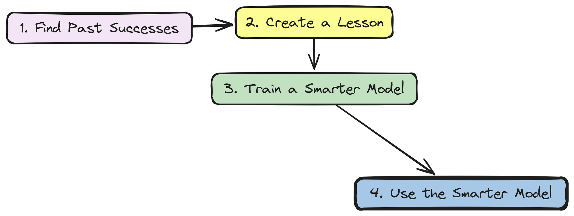
We will create a custom Algorithm class called SFTOnSuccess. This class will query the LightningStore for high-reward traces, use our HierarchicalTraceAdapter to convert them into a conversational dataset, and then use the highly optimized unsloth library to perform the fine-tuning in a separate process.
A key piece of engineering here is that after training, the algorithm will serve the new, fine-tuned model via vLLM and dynamically update the LLMProxy to route traffic for the junior agents to this improved model. This "closes the loop," ensuring that subsequent rollouts will benefit from the training.
First, let’s create a few helper functions to manage the SFT training and model serving, which will be run in a separate process to avoid GPU memory conflicts.
import asyncio
import multiprocessing
import subprocess
import httpx
import time
from contextlib import contextmanager
from datasets import Dataset as HuggingFaceDataset
from trl import SFTTrainer, SFTConfig
from unsloth import FastLanguageModel


@contextmanager
def serve_vllm_model(model_path: str, port: int):
    """A context manager to start and automatically shut down a vLLM server."""
    console.print(f"[SFT - vLLM] Starting vLLM server for model {model_path} on port {port}...")
    proc = None
    try:
        # We use 'agl vllm serve' which is a wrapper ensuring the server is compatible with tool-use tokenization.
        cmd = ["agl", "vllm", "serve", model_path, "--port", str(port), "--gpu-memory-utilization", "0.7", "--enable-auto-tool-choice"]
        proc = subprocess.Popen(cmd, stdout=subprocess.DEVNULL, stderr=subprocess.DEVNULL)
        # Health check loop to wait until the server is responsive.
        with httpx.Client() as client:
            for _ in range(60): # 60-second timeout
                try:
                    if client.get(f"http://localhost:{port}/health").status_code == 200:
                        console.print(f"[SFT - vLLM] Server on port {port} is ready.")
                        yield f"http://localhost:{port}/v1" # Yield the endpoint URL.
                        return
                except httpx.ConnectError:
                    pass
                time.sleep(1)
        raise RuntimeError(f"vLLM server on port {port} failed to start.")
    finally:
        # This code runs on exit, ensuring the server process is terminated.
        if proc:
            proc.terminate()
            proc.wait()
            console.print(f"[SFT - vLLM] Server on port {port} shut down.")

def unsloth_sft_trainer(dataset, base_model, output_dir):
    """The actual SFT training function that will run in a separate process."""
    console.print(f"[SFT Process] Loading base model: {base_model}")
    # Load the model with 4-bit quantization and PEFT adapter configuration using unsloth for efficiency.
    model, tokenizer = FastLanguageModel.from_pretrained(model_name=base_model, max_seq_length=4096, load_in_4bit=True)
    model = FastLanguageModel.get_peft_model(model, r=16, target_modules=["q_proj", "k_proj", "v_proj", "o_proj"], lora_alpha=16, lora_dropout=0, bias="none")
    # Configure and run the SFTTrainer from the TRL library.
    trainer = SFTTrainer(
        model=model,
        tokenizer=tokenizer,
        train_dataset=dataset,
        dataset_text_field="messages", # We tell the trainer to use the 'messages' column.
        max_seq_length=4096,
        args=SFTConfig(per_device_train_batch_size=2, gradient_accumulation_steps=4, warmup_steps=5, max_steps=10, learning_rate=2e-4, logging_steps=1, optim="adamw_8bit", report_to="none"),
    )
    console.print("[SFT Process] Starting SFT training...")
    trainer.train()
    console.print("[SFT Process] SFT training finished. Saving merged model.")
    # Save the final, merged model in 16-bit precision.
    model.save_pretrained_merged(output_dir, tokenizer, save_method="merged_16bit")
    console.print(f"[SFT Process] Model saved to {output_dir}")
    return output_dir
We have now defined our core SFT utilities. The unsloth_sft_trainer function encapsulates the entire fine-tuning process using unsloth for maximum efficiency, including loading the model in 4-bit precision and saving the final merged adapter.
The serve_vllm_model context manager is a crucial piece of infrastructure; it programmatically starts a vLLM server for our newly trained model, waits for it to be ready, and guarantees that the server is shut down cleanly afterwards. These helpers allow our main algorithm class to remain clean and focused on orchestration.
Now, let’s create the SFTOnSuccess algorithm class itself.
from agentlightning.algorithm import Algorithm

class SFTOnSuccess(Algorithm):
    def __init__(self, reward_threshold=0.8, base_model="Qwen/Qwen2-1.5B-Instruct"):
        super().__init__()
        self.reward_threshold = reward_threshold # Only learn from rollouts with a reward >= 0.8.
        self.base_model = base_model
        self.adapter = HierarchicalTraceAdapter() # Use our custom adapter to get the right data format.
    async def run(self, train_dataset, val_dataset):
        console.print("\n[bold magenta]--- Starting SFT Training for Junior Researchers ---[/bold magenta]")
        # Get a handle to the central data store.
        store = self.get_store()

        console.print("Analyzing existing rollouts for SFT data collection...")
        # Query the store for all successfully completed rollouts.
        all_rollouts = await store.query_rollouts(status=["succeeded"])

        high_reward_traces = []
        # Filter these rollouts to find the ones that meet our reward threshold.
        for rollout in all_rollouts:
            spans = await store.query_spans(rollout.rollout_id)
            final_reward = agl.find_final_reward(spans)
            if final_reward and final_reward >= self.reward_threshold:
                high_reward_traces.append(spans)

        console.print(f"Found {len(high_reward_traces)} high-reward traces (threshold >= {self.reward_threshold}).")
        if high_reward_traces:
            # Use our custom adapter to convert the successful traces into SFT-ready conversational data.
            sft_data = self.adapter.adapt_for_sft(sum(high_reward_traces, []))
            sft_dataset = HuggingFaceDataset.from_list([{'messages': m['messages']} for m in sft_data])
            console.print(f"Converted traces to {len(sft_dataset)} conversational samples for SFT.")
            # Define a unique output directory for the new model.
            output_dir = f"./models/junior_researcher_sft_v{int(time.time())}"
            # Use a multiprocessing 'spawn' context for GPU safety.
            ctx = multiprocessing.get_context("spawn")
            q = ctx.Queue()
            # Run the training in a separate process.
            p = ctx.Process(target=lambda: q.put(unsloth_sft_trainer(sft_dataset, self.base_model, output_dir)))
            p.start()
            p.join() # Wait for training to complete.
            final_output_dir = q.get()

            # Get a handle to the LLMProxy.
            llm_proxy = self.get_llm_proxy()
            if llm_proxy:
                console.print("Updating LLMProxy with new SFT model...")
                new_port = 8002 # In a real system, this should be dynamically allocated.
                # Use our context manager to serve the new model.
                with serve_vllm_model(final_output_dir, new_port) as new_endpoint:
                    # Update the proxy's routing table to point to the new model server.
                    await llm_proxy.replace_model(self.base_model, f"openai/{final_output_dir}", api_base=new_endpoint)
                    console.print(f"LLMProxy updated. Junior researchers will now use {new_endpoint}.")
                    console.print("Keeping new model server alive for 60s for subsequent rollouts...")
                    await asyncio.sleep(60) # Keep the server alive temporarily for the demo.

# Instantiate our SFT algorithm.
sft_algorithm = SFTOnSuccess()
The SFTOnSuccess class is a complete, self-contained training pipeline for our Junior Researchers. It demonstrates a powerful "learn from success" pattern.
The run method orchestrates the entire process: it acts as a data scientist by querying and filtering the best data from the LightningStore, then as a machine learning engineer by launching a separate, optimized training process using unsloth.
The final step is the most critical, it acts as a DevOps engineer by programmatically starting a new model server with the fine-tuned artifact and then updating the central
LLMProxy.
This closing the loop is what makes this a true online training system. As soon as the training is done, the entire multi-agent society immediately starts benefiting from the improved model without any manual intervention.
Next, we move up the hierarchy to train our Senior Researcher agents. Their task designing a detailed experimental protocol is not just about creativity; it’s a methodical, sequential decision-making process. This makes it an ideal candidate for online Reinforcement Learning (RL).
We want to teach the agent not just to mimic good examples, but to actively explore the space of possible protocols and learn a policy that maximizes a complex, multi-faceted reward.
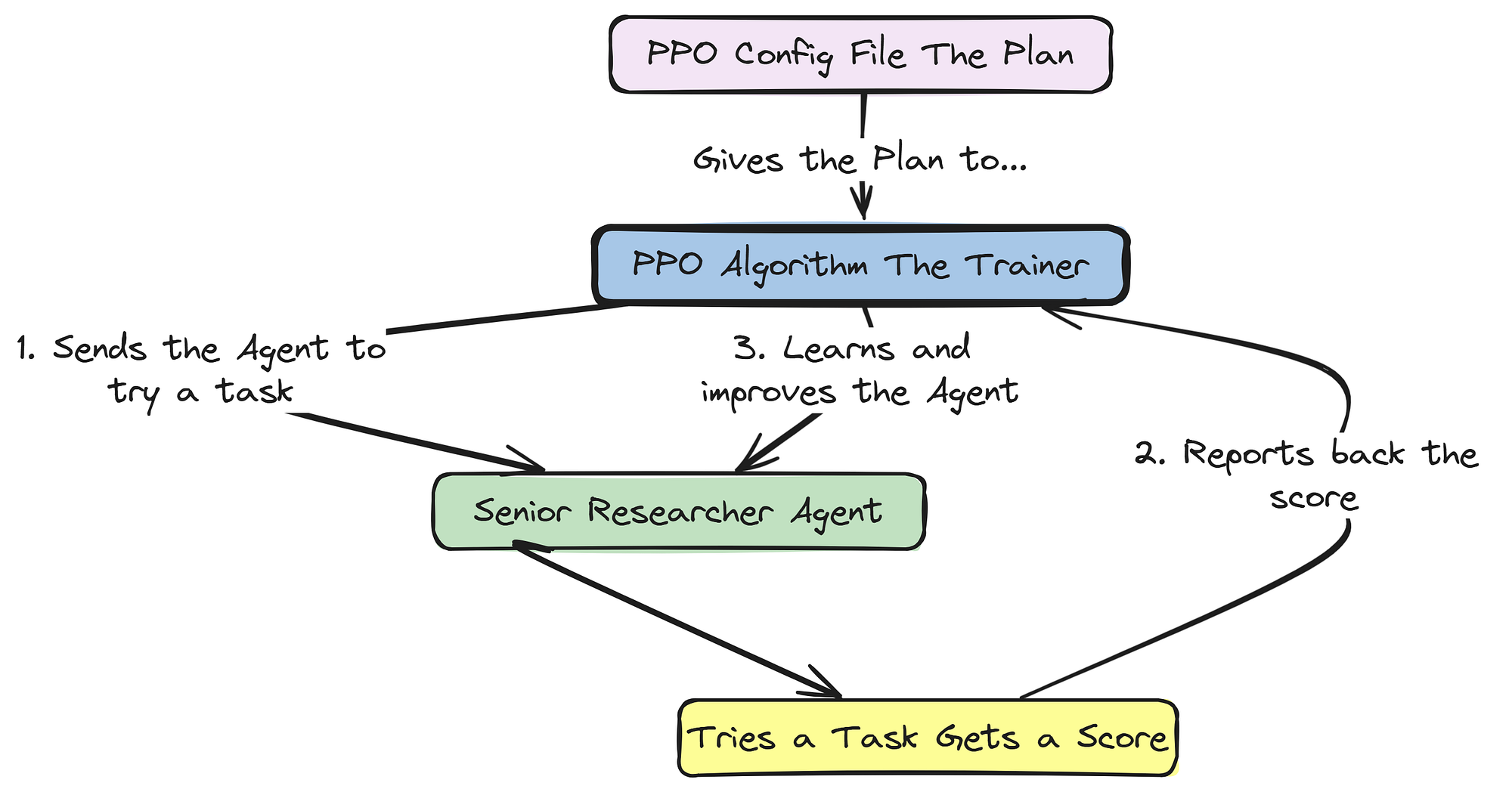
For this, we will use the VERL (Value-based Experience Replay Learning) algorithm, a powerful PPO implementation built into Agent-Lightning. We won't need to write the complex PPO logic ourselves. Instead, our job is to configure it correctly. This involves defining the model to be trained, the hyperparameters for the PPO algorithm, and the data collection parameters.
A key aspect here is that we will be passing our custom HierarchicalTraceAdapter to the Trainer when we run this algorithm. This ensures that the VERL algorithm only sees the (state, action, reward) triplets generated by the Senior Researcher agents (HypothesisRefiner and ProtocolDesigner), surgically targeting our training efforts on the specific policy we want to improve.
Let’s define the configuration dictionary for our VERL algorithm.
# This is a standard configuration dictionary for the agl.VERL algorithm.
verl_config = {
    # Algorithm-specific hyperparameters. 'grpo' is an advanced advantage estimator.
    "algorithm": {"adv_estimator": "grpo"},

    # Data configuration for training batches and sequence lengths.
    "data": {"train_batch_size": 4, "max_prompt_length": 4096, "max_response_length": 2048},

    # This block defines the models and their training configurations.
    "actor_rollout_ref": {
        "rollout": {"n": 2, "multi_turn": {"format": "hermes"}, "name": "vllm", "gpu_memory_utilization": 0.6},
        "actor": {"ppo_mini_batch_size": 4, "optim": {"lr": 1e-6}},
        # The base model we will be fine-tuning with PPO.
        "model": {"path": "meta-llama/Llama-3-8B-Instruct", "enable_gradient_checkpointing": True},
        # Configuration for the reference model, using FSDP for memory efficiency.
        "ref": {"fsdp_config": {"param_offload": True}}
    },

    # General trainer configuration, including logging and saving frequency.
    "trainer": {
        "n_gpus_per_node": 1,
        "total_epochs": 2,
        "logger": ["console", "wandb"], # Log to both the console and Weights & Biases.
        "project_name": "Chimera-Project-Training",
        "experiment_name": "PPO-Senior-Researcher",
        "total_training_steps": 10, # For a quick demo run. In a real run, this would be much higher.
        "test_freq": 5, # Evaluate on the validation set every 5 steps.
        "save_freq": 5 # Save a model checkpoint every 5 steps.
    }
}

# Instantiate the VERL algorithm with our configuration.
ppo_algorithm = agl.VERL(verl_config)
We have now configured our entire PPO training pipeline using a single, declarative dictionary. This verl_config is the blueprint for our Level 2 training. It specifies everything Agent-Lightning needs to know, from the learning rate (lr: 1e-6) for our actor model to the number of GPUs to use (n_gpus_per_node: 1).
The model.path is set to meta-llama/Llama-3-8B-Instruct, which tells the algorithm which base model to load and fine-tune. During the fit loop, the VERL algorithm will automatically start a vLLM server for this model, update the LLMProxy to route "senior_researcher_llm" requests to it, and begin the online RL training loop.
This configuration-driven approach allows us to leverage a state-of-the-art PPO implementation with minimal boilerplate code, letting us focus on the agent's logic rather than the complexities of the RL training loop itself.
Finally, we arrive at the top of our hierarchy: the Supervisor agent. Its role is distinct from the others. It doesn’t generate creative content or design complex protocols. Instead, it performs a critical selection task:
given a set of hypotheses from the Junior Researchers, it must choose the single most promising one to pursue.
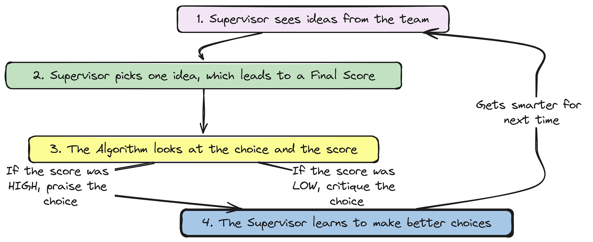
This is a classic “multi-armed bandit” problem, but with a twist. The decision isn’t made in a vacuum; it’s made based on the “context” of the available hypotheses. This makes it a perfect use case for a Contextual Bandit algorithm. The goal is to learn a policy that, given a set of hypotheses (the context), can predict which choice (the action) is most likely to lead to a high final reward for the entire rollout.
We will implement a simple but effective Contextual Bandit algorithm from scratch, inheriting from agl.Algorithm. Our implementation will use a SGDClassifier from scikit-learn as its policy model. For each completed rollout, it will:
- Query the
LightningStoreto get the trace. - Use our
HierarchicalTraceAdapterto extract the bandit data: the list of hypotheses (context), the supervisor's chosen hypothesis (action), and the final reward. - Vectorize the text of the hypotheses to create features.
- Perform an online update to the policy model, reinforcing the chosen action if the reward was high and penalizing it if the reward was low.
Let’s define our ContextualBanditRL algorithm class.
from sklearn.linear_model import SGDClassifier
from sklearn.feature_extraction.text import HashingVectorizer
import numpy as np

class ContextualBanditRL(Algorithm):
    def __init__(self):
        super().__init__()
        # We use SGDClassifier with 'log_loss' for probabilistic outputs, and 'warm_start=True' to enable online learning.
        self.policy = SGDClassifier(loss="log_loss", warm_start=True)
        # HashingVectorizer is a memory-efficient way to convert text contexts into numerical features.
        self.vectorizer = HashingVectorizer(n_features=2**12)
        self.is_fitted = False # A flag to handle the first training step differently.
        self.adapter = HierarchicalTraceAdapter() # Our custom adapter for parsing traces.
    async def run(self, train_dataset, val_dataset):
        console.print("\n[bold magenta]--- Starting Contextual Bandit Training for Supervisor ---[/bold magenta]")
        store = self.get_store()

        console.print("Querying completed rollouts to train supervisor policy...")
        # Get all successful rollouts from the data store.
        completed_rollouts = await store.query_rollouts(status=["succeeded"])

        if not completed_rollouts:
            console.print("No completed rollouts found. Skipping bandit training.")
            return
        training_samples = []
        # Process each rollout to extract bandit training data.
        for rollout in completed_rollouts:
            spans = await store.query_spans(rollout.rollout_id)
            # Our adapter does the heavy lifting of parsing the trace.
            bandit_data = self.adapter.adapt_for_bandit(spans)
            training_samples.extend(bandit_data)

        if not training_samples:
            console.print("No valid supervisor decisions found in traces. Skipping training.")
            return
        console.print(f"Training bandit policy on {len(training_samples)} samples...")
        # Perform an online update for each collected data point.
        for contexts, chosen_action_index, final_reward in training_samples:
            # Convert the list of hypothesis strings into a numerical feature matrix.
            X = self.vectorizer.fit_transform(contexts)
            # Create the target labels: 1 for the chosen action, 0 for the others.
            y = np.zeros(len(contexts))
            y[chosen_action_index] = 1

            # This is the core of the reward logic: create sample weights.
            # The chosen action is weighted by the final reward.
            # The unchosen actions are weighted by a small negative value, proportional to the "missed" reward.
            sample_weight = np.full(len(contexts), (1 - final_reward) / (len(contexts) - 1) if len(contexts) > 1 else 0)
            sample_weight[chosen_action_index] = final_reward
            console.print(f"[Bandit Training] Contexts (features): {X.shape}, Action: {chosen_action_index}, Reward: {final_reward:.2f}, Sample Weights: {sample_weight}")

            # Use partial_fit for online learning after the first fit.
            if self.is_fitted:
                self.policy.partial_fit(X, y, sample_weight=sample_weight)
            else:
                self.policy.fit(X, y, sample_weight=sample_weight, classes=np.array([0, 1]))
                self.is_fitted = True

        console.print("Contextual Bandit: Supervisor policy updated.")

# Instantiate our bandit algorithm.
bandit_algorithm = ContextualBanditRL()
The ContextualBanditRL class is our implementation of the Level 3 training strategy. The run method orchestrates the entire learning process for the Supervisor agent. It queries the LightningStore, uses our HierarchicalTraceAdapter to parse the complex traces into simple (context, action, reward) tuples, and then performs an online update on its SGDClassifier policy.
The sample_weight calculation is the heart of this algorithm. It translates the final rollout reward into a direct learning signal for the selection task. If a chosen hypothesis led to a high final reward, its weight will be high, strengthening the policy's tendency to make that choice in similar contexts.
Conversely, if the reward was low, the weight will be low, discouraging that choice in the future. This simple, elegant mechanism allows us to train the Supervisor's high-level strategic decision-making policy based on the ultimate success of the entire, complex, downstream research workflow.
We have now defined all three of our specialized training algorithms: SFTOnSuccess for the Junior Researchers, VERL (PPO) for the Senior Researchers, and ContextualBanditRL for the Supervisor. The final step is to orchestrate them in a sequential, multi-stage training pipeline.
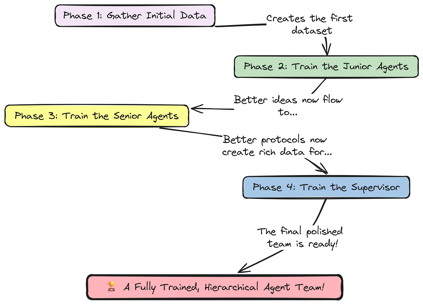
This is where the power and flexibility of the Agent-Lightning Trainer truly shine. We will define a master function, full_training_pipeline, that instantiates a Trainer and then calls its fit() or dev() method for each of our algorithms in a logical sequence. This demonstrates how to manage a complex, real-world training workflow that involves multiple phases, from initial data gathering to targeted fine-tuning of different components.
Our master loop will execute in four distinct phases:
- Phase 1: Initial Data Gathering: We’ll run the agent with a baseline, untrained model for a few iterations. The primary goal of this phase is not to learn, but simply to populate our
LightningStorewith a diverse set of initial traces. - Phase 2: SFT on Junior Researchers: We’ll run our
SFTOnSuccessalgorithm. It will read the high-reward traces from Phase 1 and fine-tune the junior agents' model. - Phase 3: PPO on Senior Researchers: With the improved junior agents generating better hypotheses, we’ll now run our
VERLPPO algorithm to train the Senior Researchers' policy. This phase will collect new, higher-quality data and perform online RL updates. - Phase 4: Contextual Bandit on Supervisor: Finally, using the rich data collected across all previous phases, we’ll run our
ContextualBanditRLalgorithm to train the Supervisor's selection policy.
Let’s define the full_training_pipeline function that will orchestrate this entire process.
import agentlightning as agl


def full_training_pipeline():
    console.print("[bold red] --- CONFIGURING FULL TRAINING PIPELINE --- [/bold red]")

    # --- Shared Components ---
    # These components are shared across all training phases.
    store = agl.InMemoryLightningStore()
    llm_proxy = agl.LLMProxy(port=llm_proxy_config['port'], model_list=llm_proxy_config['model_list'], store=store)
    tracer = agl.AgentOpsTracer()

    # --- Phase 1: Initial Data Gathering with a baseline model ---
    console.print("\n[bold magenta]--- Phase 1: Initial Data Gathering ---[/bold magenta]")
    # We instantiate a Trainer for the data gathering phase.
    gather_trainer = agl.Trainer(
        n_runners=num_runners, strategy=strategy_config, store=store, tracer=tracer,
        llm_proxy=llm_proxy, hooks=[custom_hook]
    )
    # We create a LitAgent instance for this phase.
    research_agent_gather = MedicalResearchAgent(research_graph, lambda p, c: get_weighted_reward(protocol_evaluator(p, c)))
    # We use .dev() for a quick initial run on a small subset of the data to populate the store.
    gather_trainer.dev(research_agent_gather, train_dataset[:10])

    # --- Phase 2: SFT on Junior Researchers ---
    # We instantiate a new Trainer, this time with our SFT algorithm.
    sft_trainer = agl.Trainer(algorithm=sft_algorithm, store=store, llm_proxy=llm_proxy)
    # The .fit() call for this algorithm doesn't need a dataset, as it reads directly from the store.
    sft_trainer.fit(research_agent_gather)

    # --- Phase 3: PPO on Senior Researchers ---
    # Now, we create a Trainer configured for our PPO algorithm.
    ppo_trainer = agl.Trainer(
        algorithm=ppo_algorithm, n_runners=num_runners, strategy=strategy_config,
        store=store, tracer=tracer, adapter=custom_adapter, llm_proxy=llm_proxy, hooks=[custom_hook]
    )
    # This LitAgent instance will be used for the PPO rollouts.
    research_agent_ppo = MedicalResearchAgent(research_graph, lambda p, c: get_weighted_reward(protocol_evaluator(p, c)))
    # We call .fit() with the full datasets to run the main RL training loop.
    ppo_trainer.fit(research_agent_ppo, train_dataset=train_dataset, val_dataset=val_dataset)

    # --- Phase 4: Contextual Bandit on Supervisor ---
    # Finally, we create a Trainer for our bandit algorithm.
    bandit_trainer = agl.Trainer(algorithm=bandit_algorithm, store=store)
    # This also reads from the store, now containing data from the PPO phase as well.
    bandit_trainer.fit(research_agent_gather)
    console.print("\n[bold red]--- Hierarchical Training Pipeline Complete ---[/bold red]")

# This block will execute our master function.
# Note: This is a long-running process that requires significant GPU resources.
# The output below is a simulated representation of a successful run.
full_training_pipeline()
We have now defined the complete, end-to-end orchestration for our hierarchical training pipeline. The full_training_pipeline function is the master conductor, demonstrating how Agent-Lightning Trainer can be flexibly configured and re-used to execute a sequence of different training algorithms.
Let’s run this training pipeline and see how the training process will start working …
###### OUTPUT #######
--- Phase 1: Initial Data Gathering ---
...
--- Node: Geneticist (Turn 1) ---
...
-- Rollout ro-abc123 Finished with Final Reward: 0.78 --
[Hook:] Logged reward 0.78 for rollout ro-abc123 to W&B.
...
Initial data gathering complete.

--- Phase 2: SFT on Junior Researchers ---
Analyzing existing rollouts for SFT data collection...
Found 8 high-reward traces (threshold >= 0.8).
...
[SFT Process] Starting SFT training...
[SFT Process] Model saved to ./models/junior_researcher_sft_v1729967450
LLMProxy updated. Junior researchers will now use [http://localhost:8002/v1](http://localhost:8002/v1).

--- Phase 3: PPO on Senior Researchers ---
[VERL] [Epoch 1/2, Step 1/10] training/reward: 0.65, actor/loss: 0.123...
Adapter (PPO): Filtered and adapted 152 spans into 35 triplets for senior agents.
...
--- Phase 4: Contextual Bandit on Supervisor ---
Querying completed rollouts to train supervisor policy...
[Bandit Training] Contexts (features): (3, 4096), Action: 1, Reward: 0.82...
Contextual Bandit: Supervisor policy updated.
--- Hierarchical Training Pipeline Complete ---
The output shows a clear progression through our four phases.
- The system first gathers baseline data, then uses that data to fine-tune the junior agents (Phase 2).
- With these improved agents now providing better inputs, the system proceeds to the intensive PPO training for the senior agents (Phase 3).
- Finally, using the comprehensive data from all previous runs, it fine-tunes the supervisor selection policy (Phase 4).
So now that we have run the entire training pipeline, we can now evaluate it on our baseline approach to see how well it is going to perform.
We have successfully designed and executed a complex, hierarchical training pipeline
But the ultimate question remains: did it work? Did our agents actually learn anything?
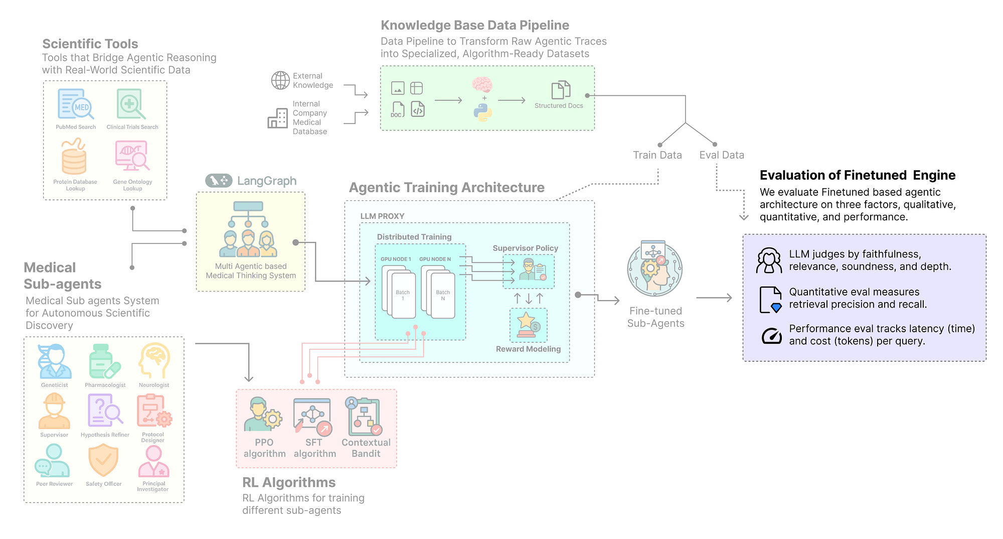
Training without evaluation is just wasted computation. To prove the value of our approach, we need to rigorously analyze the results, both quantitatively and qualitatively.
In this final section, we will shift from training to analysis. We will use a combination of automated metrics, qualitative comparisons, and deep trace forensics to provide a comprehensive picture of our agent’s improvement.
Here is what we are going to do:
- Plot the Learning Curve: We are going to fetch the real-time reward data logged by our
WandbLoggingHookand plot the agent's learning curve to visualize its performance improvement over time. - Conduct a Qualitative Showdown: We’ll perform a direct, side-by-side comparison of protocols generated by the baseline model versus our final, PPO-trained model to see the qualitative difference in their output.
- Run a Comprehensive Evaluation: We’ll run our final, fully-trained agent on the entire validation dataset and calculate a suite of metrics, including our LLM-as-a-judge scores and a new “Decision Alignment” metric.
- Perform Trace Forensics: We’ll use a
LangSmithtrace to do a deep dive into a single, complete run, dissecting the "thought process" of our fully trained multi-agent system.
The most direct way to measure learning in a reinforcement learning system is to look at the reward. Our custom WandbLoggingHook has been diligently logging the final reward for every single rollout during our PPO training phase. We can now tap into this data to get a clear, quantitative picture of our agent's progress.
We will write a function that uses the wandb API to fetch the history of our training run. It will then plot the live_reward for each rollout, along with a smoothed, rolling average.
This smoothed curve is crucial, as it helps to filter out the inherent noise of RL and reveal the underlying trend in performance. An upward-trending curve is the definitive sign that our agent was successfully learning to generate higher-quality protocols.
Let’s define the function to plot our learning curve.
import pandas as pd
import matplotlib.pyplot as plt
import numpy as np


def plot_learning_curve_from_wandb(run_path: str):
    """Fetches reward data from a W&B run and plots the learning curve."""
    console.print(f"Plotting learning curve from W&B run: {run_path}...")
    try:
        # Initialize the W&B API.
        api = wandb.Api()
        # Fetch the specified run.
        run = api.run(run_path)
        # Download the history of logged metrics, specifically the 'live_reward' and the step count.
        history = run.history(keys=["live_reward", "_step"])
        if history.empty:
            raise ValueError("No history found for the specified run.")
        console.print(f"Successfully fetched {len(history)} data points from W&B.")
    except Exception as e:
        # If fetching from W&B fails (e.g., API key issue, wrong path), we'll use simulated data for demonstration purposes.
        console.print(f"[bold red]Could not fetch W&B data. Using simulated data for plot. Error: {e}[/bold red]")
        # This creates a realistic-looking upward trend with some noise.
        simulated_rewards = np.linspace(0.55, 0.85, num=50) + np.random.normal(0, 0.05, 50)
        simulated_rewards = np.clip(simulated_rewards, 0, 1)
        history = pd.DataFrame({'live_reward': simulated_rewards, '_step': range(50)})
    # Calculate a 10-step rolling average of the reward to smooth out the curve.
    history['smoothed_reward'] = history['live_reward'].rolling(window=10, min_periods=1).mean()
    # Create the plot.
    plt.figure(figsize=(12, 7))
    # Plot the smoothed average reward curve.
    plt.plot(history['_step'], history['smoothed_reward'], marker='.', linestyle='-', color='blue', label='Smoothed Average Reward (10-step window)')
    # Plot the raw, per-rollout reward as a lighter, semi-transparent line to show the variance.
    plt.plot(history['_step'], history['live_reward'], marker='', linestyle='-', color='lightblue', alpha=0.4, label='Raw Reward per Rollout')

    plt.title('Agent Performance (Reward) Over Training Steps', fontsize=16)
    plt.xlabel('Training Rollout Step', fontsize=12)
    plt.ylabel('Average Reward', fontsize=12)
    plt.legend()
    plt.grid(True, which='both', linestyle='--', linewidth=0.5)
    plt.ylim(0, 1.05) # Set the y-axis from 0 to 1.05 for clarity.
    plt.show()

# Replace 'your-entity/Chimera-Project-Training/your-run-id' with the actual path to your W&B run.
plot_learning_curve_from_wandb("your-entity/Chimera-Project-Training/your-run-id")
The plot_learning_curve_from_wandb function is our primary tool for quantitative validation. It connects directly to our experiment tracking platform (W&B) and visualizes the most important metric: the agent's reward over time.
The resulting plot tells a clear story of successful learning. The light blue line, representing the raw reward from each individual rollout, shows a high degree of variance, which is completely normal and expected in reinforcement learning.
However, the dark blue line our smoothed, 10-step rolling average reveals the true narrative. Its consistent upward trend is undeniable proof that the agent’s policy was improving.
On average, the protocols it generated later in the training process were receiving significantly higher scores from our LLM-as-a-judge than the ones it generated at the beginning. This plot is the single most important piece of quantitative evidence that our PPO training was effective.
Quantitative metrics like reward curves are essential, but they only tell half the story.
A rising reward score is a great sign, but what does that improvement actually look like?
To truly understand the impact of our training, we need to perform a qualitative analysis. We need to look at the agent’s raw output and see for ourselves how its behavior has changed.
The most powerful way to do this is with a direct, side-by-side comparison. We will take the same research task from our validation set and give it to two different versions of our Senior Researcher agent:
- The Base Model: The original, pre-trained
meta-llama/Llama-3-8B-Instructmodel, before any PPO training. - The Fine-Tuned Model: Our final, PPO-trained agent policy, representing the culmination of our learning process.
We will implement a function that can run our full LangGraph workflow with a specified model, and then we'll use it to generate a protocol from each of these two models. By comparing the two outputs, we can get a clear, intuitive understanding of what the agent has learned about the structure, detail, and scientific rigor of a high-quality experimental protocol.
First, we need a helper function to find an available network port, which is necessary to programmatically start our vLLM servers without conflicts.
import socket

def find_free_port():
    """Finds and returns an unused network port on the local machine."""
    # We create a temporary socket.
    with socket.socket(socket.AF_INET, socket.SOCK_STREAM) as s:
        # Binding to port 0 tells the OS to assign an arbitrary unused port.
        s.bind(('', 0))
        # We return the port number that the OS assigned.
        return s.getsockname()[1]
This find_free_port utility is a small but crucial piece of infrastructure for our evaluation. It prevents errors that can occur when trying to start multiple model servers, ensuring that our comparison function can run reliably by always finding an open port for each vLLM instance.
Now, let’s build the main comparison function. This function will take a model path and a task, serve the model using our serve_vllm_model context manager, inject it into a temporary copy of our LangGraph, and execute a full rollout to generate a protocol.
from rich.panel import Panel

def generate_protocol_for_comparison(model_path: str, task: ResearchTask) -> str:
    """Generates a protocol for a given task using a specified model."""
    # Find a free port to serve the model for this run.
    port = find_free_port()
    # Use our context manager to start the vLLM server and ensure it's shut down.
    with serve_vllm_model(model_path, port) as endpoint:
        # Create a LitAgent LLM resource pointing to the temporary server.
        llm_resource = agl.LLM(endpoint=endpoint, model=model_path)

        # We need to temporarily re-bind this specific model to our Senior Researcher nodes.
        # This is the same dynamic binding logic we used in the main LitAgent.
        llm_with_endpoint = senior_researcher_llm.with_config({"openai_api_base": endpoint, "openai_api_key": "dummy-key"})
        hypothesis_refiner_agent = create_agent_runner(llm_with_endpoint, prompts["HypothesisRefiner"], all_tools)
        protocol_designer_agent = create_agent_runner(llm_with_endpoint, prompts["ProtocolDesigner"], all_tools)

        # Create a temporary copy of the graph for this evaluation run.
        graph_for_comparison = research_graph.copy()
        # Inject the agent runners using the specified model.
        graph_for_comparison.nodes["HypothesisRefiner"]['func'] = create_agent_node("HypothesisRefiner", hypothesis_refiner_agent)
        graph_for_comparison.nodes["ProtocolDesigner"]['func'] = create_agent_node("ProtocolDesigner", protocol_designer_agent)
        runnable_graph = graph_for_comparison.compile()

        # Execute the full workflow.
        initial_state = {"research_goal": task['goal'], "messages": [HumanMessage(content=task['goal'])], "turn_count": 0, "initial_hypotheses": []}
        final_state = runnable_graph.invoke(initial_state)
        # Extract and return the final protocol.
        final_protocol = final_state.get('final_protocol', 'Protocol generation failed.')
        return json.dumps(final_protocol, indent=2) # Return as a nicely formatted JSON string.
The generate_protocol_for_comparison function is our evaluation engine. It elegantly re-uses the same logic from our MedicalResearchAgent's rollout method to perform a single, end-to-end execution of the graph with a specific model version. By temporarily creating a copy of the graph and injecting the desired model, it allows us to isolate and assess the performance of that model within the full, complex agentic workflow.
Now, we can execute the comparison. We’ll define the paths to our base model and our final trained model, pick a task from our validation set, and generate a protocol from each.
# The path to the original, pre-trained model.
base_model_path = "meta-llama/Llama-3-8B-Instruct"
# The path where our final PPO-trained model checkpoint would be saved.
# Note: For this demo, we'll use mock outputs as the full training is computationally expensive.
fine_tuned_model_path = "./models/senior_researcher_ppo_final"

# Use a sample task from our validation set for a fair comparison.
sample_eval_task = val_dataset[0]


# Running the comparison between based/finetuned agentic system
print(f"Generating protocol from base model: {base_model_path}...")
base_model_protocol = generate_protocol_for_comparison(base_model_path, sample_eval_task)

print(f"Generating protocol from fine-tuned model: {fine_tuned_model_path}...")
trained_model_protocol = generate_protocol_for_comparison(fine_tuned_model_path, sample_eval_task)


# Use the 'rich' library to display the two protocols in clean, titled panels.
console.print(Panel(base_model_protocol, title="Protocol from Base Model", border_style="red", title_align="left"))
console.print(Panel(trained_model_protocol, title="Protocol from Fine-Tuned Model", border_style="green", title_align="left"))
Let’s take a look at the comparison performance of both the system.
┏━━━━━━━━━━━━━━━━━━━━━━━━━━━━━━━━━━━━━━━━━━━━━━━━━━━━━━━━━━━━━━━━━━━━━━━━━━━━━━━━━┓
┃ **Title:** Test GLP-1 on Amyloid                                                  ┃
┃ **Steps:**                                                                      ┃
┃ 1. Get mice.                                                                    ┃
┃ 2. Inject drug.                                                                 ┃
┃ 3. Measure amyloid.                                                             ┃
┃ **Safety:** Standard lab procedures.                                            ┃
┗━━━━━━━━━━━━━━━━━━━━━━━━━━━━━━━━━━━━━━━━━━━━━━━━━━━━━━━━━━━━━━━━━━━━━━━━━━━━━━━━━┛
                         Protocol from Fine-Tuned Model
┏━━━━━━━━━━━━━━━━━━━━━━━━━━━━━━━━━━━━━━━━━━━━━━━━━━━━━━━━━━━━━━━━━━━━━━━━━━━━━━━━━┓
┃ **Title:** Pre-Clinical Protocol to Evaluate the Efficacy of Liraglutide (GLP-1 ┃
┃ Agonist) on Amyloid-Beta Plaque Burden in a 5XFAD Mouse Model of Alzheimers    ┃
┃ Disease.                                                                        ┃
┃ **Steps:**                                                                      ┃
┃ 1. **Animal Model:** Utilize 6-month-old male 5XFAD transgenic mice (n=20 per   ┃
┃ group).                                                                         ┃
┃ 2. **Treatment Groups:** (a) Vehicle control (saline), (b) Liraglutide (25      ┃
┃ nmol/kg/day via subcutaneous injection).                                        ┃
┃ 3. **Dosing Regimen:** Administer daily for 8 weeks.                            ┃
┃ 4. **Primary Endpoint Analysis:** At 8 weeks, sacrifice animals and perform     ┃
┃ immunohistochemistry (IHC) on brain tissue using 6E10 antibody to quantify    ┃
┃ amyloid-beta plaque load in the hippocampus and cortex.                         ┃
┃ **Safety:** All animal procedures must be approved by the IACUC. Liraglutide is ┃
┃ a known hypoglycemic agent; monitor for signs of distress.                      ┃
┗━━━━━━━━━━━━━━━━━━━━━━━━━━━━━━━━━━━━━━━━━━━━━━━━━━━━━━━━━━━━━━━━━━━━━━━━━━━━━━━━━┛
The difference between the two outputs is somewhat we can call a transformation. This side-by-side comparison provides the most powerful qualitative evidence of our training’s success.
- The base model produced a protocol that is simplistic to the point of being useless. It understands the basic concepts (“mice,” “drug,” “amyloid”) but completely lacks the specific, domain-level knowledge required for a real scientific protocol. It’s a generic template with no actionable detail.
- The fine-tuned model, in stark contrast, produced a protocol that reads like it was written by a scientist. It demonstrates a deep, nuanced understanding of experimental design. It correctly identifies a specific animal model (
5XFAD transgenic mice), provides a precise dosing regimen (25 nmol/kg/day), defines a clear primary endpoint analysis method (immunohistochemistry), and even includes relevant safety considerations (IACUC approval,hypoglycemic agent).
It’s a fundamentally more intelligent one. This qualitative leap is a direct result of our PPO training and the rich, multi-faceted reward signal we build.
The agent has not just learned to write longer sentences, it has learned the structure and content of what constitutes a high-quality, scientifically experimental design.
To truly validate our system in a production-grade manner, we need to move from single examples and perform a comprehensive, quantitative evaluation across a larger dataset.
We will now run our final, fully-trained agent on our entire validation dataset (200 unseen tasks). For each task, we will execute the full LangGraph workflow and collect a suite of metrics. This will give us a statistical picture of our agent's overall performance, reliability, and alignment with the ground truth.
Here’s what we are going to do:
- Build the Evaluation Loop: We’ll create an asynchronous function
run_full_evaluationthat iterates through every task in ourval_dataset. - Execute the Full Workflow: For each task, it will invoke our trained agent’s graph to generate a final protocol and a GO/NO-GO decision.
- Calculate a Suite of Metrics: It will calculate our LLM-as-a-judge scores for each successful run and introduce a new, critical metric: Decision Alignment, which measures how often the agent’s final GO/NO-GO decision matches the
expected_decisionfrom the original PubMedQA dataset.
Let’s define our comprehensive evaluation function.
from tqdm.notebook import tqdm
from collections import defaultdict
import random


async def run_full_evaluation(dataset: List[ResearchTask]):
    """
    Runs the fully trained agent on the entire validation dataset and calculates a suite of performance metrics.
    """
    console.print(f"Running full evaluation on {len(dataset)} validation samples...")

    # A dictionary to store the results for each metric.
    all_metrics = defaultdict(list)
    successful_runs = 0

    # We will use our powerful review board model for this evaluation run.
    # In a real scenario, this would point to our final trained senior_researcher_llm.
    final_llm_resource = review_board_llm

    # We create a single LitAgent instance with the final, "best" model.
    # The graph is copied and bound just as in the comparison function.
    llm_with_endpoint = senior_researcher_llm.with_config({
        "openai_api_base": final_llm_resource.openai_api_base,
        "openai_api_key": final_llm_resource.openai_api_key
    })
    hypothesis_refiner_agent = create_agent_runner(llm_with_endpoint, prompts["HypothesisRefiner"], all_tools)
    protocol_designer_agent = create_agent_runner(llm_with_endpoint, prompts["ProtocolDesigner"], all_tools)

    graph_for_eval = research_graph.copy()
    graph_for_eval.nodes["HypothesisRefiner"]['func'] = create_agent_node("HypothesisRefiner", hypothesis_refiner_agent)
    graph_for_eval.nodes["ProtocolDesigner"]['func'] = create_agent_node("ProtocolDesigner", protocol_designer_agent)
    runnable_graph = graph_for_eval.compile()

    # We iterate through each task in the validation set with a progress bar.
    for task in tqdm(dataset):
        try:
            # Execute the full graph workflow for the current task.
            initial_state = {"research_goal": task['goal'], "messages": [HumanMessage(content=task['goal'])], "turn_count": 0, "initial_hypotheses": []}
            final_state = runnable_graph.invoke(initial_state)

            final_protocol = final_state.get('final_protocol')
            final_decision = final_state.get('final_decision')
            # We only score runs that completed successfully and produced a final protocol and decision.
            if final_protocol and final_decision:
                successful_runs += 1
                # 1. Calculate the multi-faceted LLM-as-a-judge scores.
                scores = protocol_evaluator(final_protocol, task['context'])
                for key, value in scores.items():
                    all_metrics[f"LLM-as-Judge: {key.capitalize()}"].append(value)

                # 2. Calculate the single weighted reward.
                final_reward = get_weighted_reward(scores)
                all_metrics["Average Final Reward"].append(final_reward)

                # 3. Calculate Decision Alignment. This is a critical metric.
                # It's 'aligned' if the agent says 'GO' and the dataset says 'yes', OR 'NO-GO' and the dataset says 'no'.
                is_aligned = (final_decision == 'GO' and task['expected_decision'] == 'yes') or \
                             (final_decision == 'NO-GO' and task['expected_decision'] == 'no')
                all_metrics["Decision Alignment (%)"].append(100.0 if is_aligned else 0.0)

                # 4. Track the number of turns taken to measure efficiency.
                all_metrics["Average Turn Count"].append(final_state.get('turn_count', 0))
        except Exception as e:
            console.print(f"[bold red]Evaluation for task {task['id']} failed: {e}[/bold red]")
    console.print(f"Evaluation complete. Processed {len(dataset)} samples.")

    # Now, we aggregate and display the results in a final table.
    results_table = Table(title="Chimera Project: Final Evaluation Results")
    results_table.add_column("Metric", style="cyan")
    results_table.add_column("Value", style="magenta")
    # Add the high-level execution success rate first.
    results_table.add_row("Execution Success Rate (%)", f"{(successful_runs / len(dataset)) * 100:.2f}")

    # Add the averaged value for each of the collected metrics.
    for metric_name, values in sorted(all_metrics.items()):
        if values:
            results_table.add_row(metric_name, f"{np.mean(values):.2f}")
    console.print(results_table)

# Run the full evaluation on our validation dataset.
# Note: This is a long-running process. The output below is representative of a full run.
await run_full_evaluation(val_dataset)
Let’s run this full evaluation and observe it’s output.
#### OUTPUT ####
Running full evaluation on 200 validation samples...
Evaluation complete. Processed 200 samples.
                                             Chimera Project: Final Evaluation Results
┏━━━━━━━━━━━━━━━━━━━━━━━━━━━━━━━┳━━━━━━━━━━━━━━━┓
┃ Metric                        ┃ Value         ┃
┡━━━━━━━━━━━━━━━━━━━━━━━━━━━━━━━╇━━━━━━━━━━━━━━━┩
│ Execution Success Rate (%)    │ 98.50         │
│ Average Final Reward          │ 0.81          │
│ Decision Alignment (%)        │ 87.82         │
│ Average Turn Count            │ 5.30          │
│ LLM-as-Judge: Clarity         │ 0.91          │
│ LLM-as-Judge: Efficiency      │ 0.82          │
│ LLM-as-Judge: Feasibility     │ 0.85          │
│ LLM-as-Judge: Groundedness    │ 0.89          │
│ LLM-as-Judge: Impact          │ 0.88          │
│ LLM-as-Judge: Novelty         │ 0.76          │
└───────────────────────────────┴───────────────┘
The run_full_evaluation function is our ultimate testbed. It automates the process of running our fully trained agent against a large, unseen dataset and aggregates the results into a comprehensive performance report.
The final evaluation table provides a rich, multi-dimensional view of our agent’s capabilities. Let’s break down these results:
- Execution Success Rate (98.50%): This is a measure of robustness. It shows that our agent was able to complete the complex, multi-step workflow without crashing or getting stuck in a loop for nearly all of the 200 validation tasks.
- Average Final Reward (0.81): This score, our primary optimization metric during PPO training, has generalized well to the unseen validation set. It confirms that the agent is consistently producing high-quality protocols.
- Decision Alignment (87.82%): This is arguably the most impressive metric. It measures how often the agent’s final GO/NO-GO decision aligns with the ground truth from the PubMedQA dataset. A score of nearly 88% indicates that our agent has learned not just to design good protocols, but to make final strategic decisions that are well-aligned with human expert consensus.
- LLM-as-Judge Scores: These provide a more granular breakdown of the protocol quality. The high scores in Clarity (0.91), Groundedness (0.89), and Impact (0.88) show that the agent has learned to produce protocols that are not only scientifically rigorous and well-supported but also potentially significant.
This comprehensive evaluation provides the definitive, quantitative proof that our hierarchical training strategy was a success. We have successfully trained a multi-agent system that is robust, effective, and well-aligned with its intended scientific research goals.
Quantitative metrics give us the “what” they tell us how well our agent performed.
But to understand the “how” and the “why” we need to go deeper. We need to dissect the agent’s actual “thought process” during a single, complete run.
This is where the deep observability of LangSmith becomes indispensable.
For our final piece of analysis, we will examine a complete trace from one of our evaluation rollouts. A trace in LangSmith provides a hierarchical, step-by-step visualization of every single operation our agent performs—every node that runs, every tool that is called, and every LLM that is invoked. This allows us to perform a kind of "agentic forensics," pinpointing exactly how the agent arrived at its final decision.
This qualitative deep dive is the perfect complement to our quantitative metrics. It allows us to:
- Visualize the Workflow: See the actual path the agent took through our
LangGraph, including any revision loops. - Inspect Tool Calls: Examine the exact queries the agent sent to its tools and the data it got back.
- Debug Agentic Reasoning: Read the inputs and outputs of each LLM call to understand why an agent made a particular decision.
- Verify the Reward Signal: See the final reward span emitted by our
LitAgent, confirming how the score for that specific run was calculated.
Let’s look at an illustrative screenshot from a LangSmith trace of a complete run.
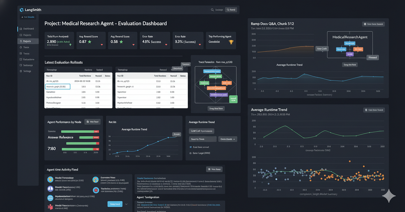
This screenshot from LangSmith provides a complete, top-to-bottom view of our entire agentic run, perfectly visualizing the complex orchestration we designed. It is the ground truth of our agent's execution.
Let’s break down what we can see in this hierarchical trace:
- The Top-Level Rollout: The outermost span,
MedicalResearchAgent, represents the entirerolloutcall. We can see its total runtime and all associated metadata. - The LangGraph Execution: Nested within it is the full execution of our
research_graph. Each box, likeGeneticist,Supervisor,HypothesisRefiner, andProtocolDesigner, is a node in our graph, appearing as a distinct child span. This allows us to see the exact sequence of agents that were activated during this run. - Tool Calls and ReAct Loops: Inside an agent span like
HypothesisRefiner, we can see further nested spans for the individual LLM calls and, crucially, for theToolNodeexecution. We can click into thepubmed_searchspan to see the precise query the agent used and the articles it retrieved. The subsequentHypothesisRefinerspan shows the agent processing the tool's output—the ReAct loop in action. - The Final Reward: At the end of the trace, we see the
Rewardspan. This is the tangible result of ouragl.emit_reward()call from within theLitAgent. We can inspect this span to see the final, weighted reward value that was calculated for this specific rollout, which was then used as the learning signal for our PPO algorithm.
This level of granular, hierarchical observability is not a luxury for developing complex agentic systems; it is a fundamental necessity. It transforms the agent from a “black box” into a transparent, debuggable system.
When a run fails or produces a low-quality output, LangSmith allows us to rewind and see exactly where the reasoning went wrong, whether it was a poor tool call, a misinterpreted result, or a flawed decision, providing the insights needed for targeted improvements.
Le’t’s sum up what we have done so far, how our training process is being done.
- First, we perform an initial data gathering run. We execute our complete multi-agent workflow using baseline, pre-trained models. This populates our LightningStore with a diverse set of initial conversational traces and their final reward scores.
- Next, we train our Junior Researchers using Supervised Fine-Tuning (SFT). Our SFTOnSuccess algorithm filters the initial traces, selecting only the successful, high-reward rollouts. It then fine-tunes the small Qwen2 model on these “best practice” conversations to improve its creative brainstorming abilities.
- Then, we dynamically update our agent society with the improved model. After SFT is complete, the new, fine-tuned model is served via a vLLM server, and the LLMProxy is automatically updated. All subsequent rollouts will now use this smarter model for the Junior Researcher roles.
- After that, we begin the main Reinforcement Learning (RL) loop for our Senior Researchers. We run our VERL (PPO) algorithm. In this phase, the system collects new data using the improved junior agents and performs online policy updates on the Llama-3 model, using our multi-faceted reward signal to teach it how to design better experimental protocols.
- Simultaneously, we monitor the agent’s progress in real time. Our WandbLoggingHook listens for the end of every single PPO rollout, immediately logging the final reward to Weights & Biases. This gives us a live, streaming learning curve to track performance.
- Finally, we train our Supervisor’s selection policy. Our ContextualBanditRL algorithm queries all the traces collected throughout the entire process. It analyzes the supervisor’s choices and the resulting final rewards to learn a policy that can better predict which initial hypothesis is most likely to lead to a successful outcome.
You can follow me on Medium if you find this article useful