Heart-Disease-Detection-using-Lab-Report-Data

---

Live Demo

Heart Diseases Detection

Underlying Biology

---

Screenshot of Application

Detailed Presentation

Presentation

Dataset

Dataset Used

Introduction

What is Heart Disease? Heart Disease is a group of conditions that affect the structure and functions of our heart. Build up of fatty material can cause arteries to narrow which prevents the heart from getting enough blood.

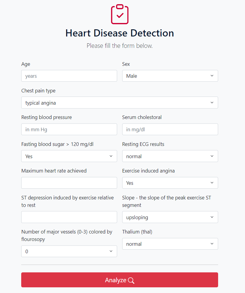
Using machine learning, our goal is to be able to predict if a patient has Heart Disease with a high degree of accuracy.

The data used is the Heart Disease Data Set from UCI Machine Learning Repository: https://archive.ics.uci.edu/ml/datasets/heart+Disease This data consists of 14 attributes. They come from 4 different locations. For this study, the dataset from Cleveland will be used.

The collection of the data is credited to the following individuals: Hungarian Institute of Cardiology. Budapest: Andras Janosi, M.D. University Hospital, Zurich, Switzerland: William Steinbrunn, M.D. University Hospital, Basel, Switzerland: Matthias Pfisterer, M.D. V.A. Medical Center, Long Beach and Cleveland Clinic Foundation:Robert Detrano, M.D., Ph.D.

Data Cleanup

Load libraries and data

# Load packages
library('ggplot2') # visualization
library('caret')
library('dplyr')
library('Hmisc')

data=read.csv('cleveland_heart.csv', header = TRUE, na.strings = c("?",""))

Check data

str(data)

We are going to consider any number 1 or greater for HEART_DISEASE as someone with heart disease so lets convert all numbers greater than 1 to 1.

data$HEART_DISEASE[data$HEART_DISEASE > 0] <- 1

Change variables to correct data type

names <- c('SEX','CHEST_PAIN','FASTING_BLOOD_SUGAR','REST_ECG','EXERCISE_INDUCED_ANGINA','SLOPE','MAJOR_VESSELS','THAL','HEART_DISEASE')
data[,names] <- lapply(data[,names] , factor)
str(data)

Drop rows with missing values (only 6)

sum(is.na(data))
data <- na.omit(data)

Visualize Data

Data Exploration

levels(data$SEX) = c("Female","Male","")
mosaicplot(data$SEX ~ data$HEART_DISEASE, main="Heart Disease by Gender", color=TRUE,
           xlab="Gender", ylab="Heart disease")

Seems like a much higher percentage of men have heart disease

ggplot(data, aes(x=AGE, color=HEART_DISEASE)) +
  geom_histogram(fill="black", alpha=0.8)

Around age 60, there seems to be a higher percentage of people with Heart disease

Correlation analysis

d2 <- data[,c(4,5,8)] # a data frame that only contains the numerical attributes
cm <- rcorr(as.matrix(d2)) # the correlation matrix with significance values
cm # this outputs the correlation matrix (r), n (which is the number of observations)
cm$P # this outputs the p values

We can say with 95% confidence than Resting Blood Pressure (rest_bp) and Cholesterol have significant correlation. This is because the p-value for rest_bp and cholesterol is 0.0234 which is less than 0.05 (5%).

Outlier Analysis

Boxplots

The boxplots for the four numerical attributes will now be plotted

boxplot(data$REST_BP, main="REST BP")
boxplot(data$CHOLESTEROL, main="CHOLESTEROL")
boxplot(data$MAX_HEART_RATE, main="MAX HEART RATE")
boxplot(data$OLDPEAK, main= "Old PEAK")

###Outlier removal and Outlier Percentile Capping

Both outlier removal and percentile capping lead to the reduction of accuracy of the model. It’s possible that the outliers are not that far off from the rest of the data thus their exclusion has a negative effect on the accuracy.

Prediction

Split into training & test sets

Data will be split into 70% Train and 30% Test. The ratio of Heart Disease is preserved in both Train and Test Data.

inTrain <- createDataPartition(data$HEART_DISEASE, times = 1, p = 0.7, list = FALSE)
trainData<-data[inTrain,]
testData<-data[-inTrain,]

Create Model

Create a model using logistic regression.

set.seed(11)
model <- glm(HEART_DISEASE ~.,family=binomial(link='logit'),data=trainData)

Model Analysis

summary(model)
anova(model,test="Chisq")

We can say with 95% confidence that the attributes (for which the p-values are less than 0.05) have a significant effect one the model.

Prediction

predicted <- plogis(predict(model, testData)) 

Check prediction accuracy

fitted.results <- ifelse(predicted > 0.5,1,0)
misClasificError <- mean(fitted.results != testData$HEART_DISEASE)
print(paste('Accuracy',1-misClasificError))

The model achieved accuracy of between 80-86%

Confusion Matrix

confMat <- confusionMatrix(factor(fitted.results, levels = 0:1),factor(testData$HEART_DISEASE, levels = 0:1))
confMat

Conclusion

A dataset of 300 patients containing 14 attributes is used to develop a Logistic Regression model to detect Heart Disease.

With the accuracy achieved, the model may be used by assist Doctor but should not be the only source to determine diagnosis.

However, this study suggests that the accuracy can be further improved with the following techniques:

1. Collect more patient data. With only 300 subjects, we achieved a relatively accurate model. It is likely that even higher accuracy can be achieved with a larger data set.
2. Try other classifiers like Neural Networks, Support Vector Machines, Decision Trees etc. and compare results.

It is recommended that the model be deployed to software used by Doctors. It can be used to quickly identify patients with Heart Disease and bring the list of patients with probable Heart Disease to the Doctors attention for further review. This will result in time and cost savings and better overall patient health in the long term.