Setting up a network

Definition of a network

As mentioned in Basic commands, <au.s>* files should include a definition of each node in the neural network to be simulated. Below we explain in more detail how individual nodes are defined, as well as describe the computational data structures that are behind a node and a connecting weight in an LSNM network.

Commands

The following commands are available to define network nodes within a neural network:

• SET: Creates a new network module.

• #INCLUDE: Reads specifications from external file.

• RUN: Runs simulation for specific number of iterations.

• CONNECT: Connects one module to the other by using the specified pattern of connections.

Object properties for the command SET

• ACTRULE (ActRule): Possible values are: Clamp, clamp activations to set values; SigAct, non-differential style sigmoid rule in which a new activation is just a sigmoid of the difference between input and threshold; DiffSig, differential equation-style sigmoid activation which adds sigmoid of the input-threshold difference to old activation and subtracts from it the product of decay and old activation; Lin, linear activation rule; Noise, noisy clamp; Sigm, sigmoidal activation; Shift, shifting activation rule which shifts the clamped activation by dx every delta iterations (useful for learning invariance of position of an object).

• INPUTRULE: In case of input rules. Not implemented.

• LEARNRULE (LearnRule): Possible values are: Off, no learning; Aff, afferent hebbian; Eff, efferent hebbian.

• OUTPUTRULE (OutputRule): Possible values are: C; SumOut.

• NODEACT (Node Activation): Initialize activation values. Possible values: ALL, all nodes;

• BINACT: Initial activation values, set by input matrix

• PHASE: Initial phase values. Possible values: ALL.

• PARAMETER (Parameters): Set parameter values. Possible values: ALL.

• LEARNPARAM: Learning rule parameter values. Possible values: ALL, learn all parameters.

• SHIFT: Explicitly shift activations

• TOPOLOGY (Topology): Specifies the network topology. Possible values: LINEAR, linear topology; RECT, rectangular topology.

• WRITEOUT (Write): Set file output to every i iterations.

• WRITEWEIGHTS (WW): Set weight writeout output to every i iterations

Object properties for the command #INCLUDE

The only parameter here is the name of the file.

Object properties for the command RUN

The only parameter here is the number of iterations.

Object properties for the command CONNECT

• FROM (From)

Data structures

The global data structure used in the programming of LSNM is illustrated below:

where NodeSet is a set of nodes that can be called a module. Initially, there is reserved space for up to max number of modules. Every module has its properties plus a pointer to the actual array of nodes that compose that structure. This nodes are of type NodeStruct and can be of different lengths (although in the current models this number is the same for all modules). Each node of the module contains its own specification plus pointers to the weights to which is connected, thereby affecting other nodes in any location of the network. WeightStruct is the data structure for a connection weight between two modules. Every connection weight contains its own set of specifications plus a pointer to the node to which it affects.

Note: only functions that are relevant to visual and auditory delayed match-to-sample simulations are defined below.

The structure of a module in the network (Pointer values are located at the right and non-pointer values are located at the left) is shown below (please note that some of the pointers are actually pointing to 'methods' in the object-oriented-programming sense:

The pointer values that make up this structure are as follows:

• Sfs: Points to a file

• Wtfs: Points to a weight file

• Params: LrnParams

• Vars

• InitSet: Points to method 'InitSet'

• OutputRule: Points to method 'OutputRule'

• InputRule: Points to method 'InputRule'

• ActRule: Points to method 'ActRule'

• Update: Points to method 'Update'

• LearnRule: Points to method 'Learnrule'

• Node: Points a dynamic vector of nodes

The non-pointer values that make up this structure are as follows:

• SetName: Character string containing structure name

• SetIndex

• WriteOut: How frequently the state of the structure is written to an output file

• WriteWts: How frequently the weights of the structure is written to an output file

• Topology: Network topology

• Xdim: Number of elements along the x axis of matrix

• YDim: Number of elements along the y axis of matrix

• NSetParams

• NLrnParams

• NSetVars

• N_Nodes: Number of nodes in this structure

Every node of the structure described above is a structure of the type NodeStruct.

The figure below illustrates the structure of a node in each module of the network (Pointer values are located at the right and non-pointer values are located at the left.)

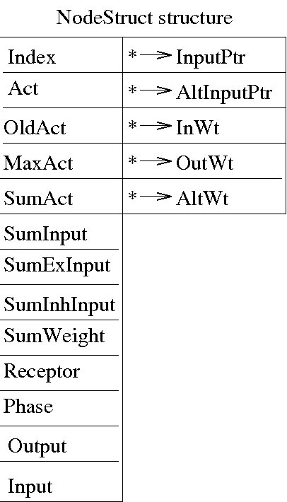
The pointer values that make up this structure are as follows:

• InputPtr

• AltInputPtr

• InWt: Points to a weight class

• OutWt

• AltWt

The non-pointer values that make up this structure are as follows:

• Index: Index of the current node

• Act

• OldAct

• MaxAct

• SumAct

• SumInput

• SumExInput

• SumInhInput

• SumWeight

• Receptor

• Phase

• Output

• Input

The structure of each of the weights interconnecting the modules of the network (Pointer values are located at the right and non-pointer values are located at the left.) is illustrated below:

The pointer values that make up this structure are as follows:

• Set
• DestNode

The non-pointer values that make up this structure are as follows:

• LearnOn
• Value
• WtVar

How to define a network

The following example illustrates the use of the command SET. In this example, the MGN module was defined for the auditory model (taken from auseq.s, a script file for the sequences memory model):

set(MGNs,81) {
  Write 5
  Topology: Rect(1,81)
  ActRule: Clamp
  OutputRule: SumOut
  Node Activation { ALL 0.01 }
}

The command set creates a new structure called MGNs, consisting of 81 nodes, and initializes all of the structures' elements to zero. The instruction Write 5 indicates that the state of each of the 81 nodes will be recorded in an output file every 5 iterations. The instruction Topology: Rect(1,81) sets the topology of the network to a vector of one column by 81 rows.

The following example illustrates how to use the commands #INCLUDE and RUN (taken from auseq.rs, a script file for the sequences memory model):

#include noinp_au.inp
Run 200 		% <----------- 1000 ms

The following example shows the first few lines of a network connection specifications (taken from mgnsea1d.w, a file containing connection weights between MGN and the excitatory part of down-selective Ai of the sequences memory model):

Connect(mgns, ea1d)  {
  From:  (1, 1)  {
    ([ 1,81]  0.047928)     ([ 1, 1]  0.099059)     |              | 
}

This example file of specification of connection weights was generated by the command netgen. The command netgen takes a *.ws file and generates the connection code. The original file of corresponding to the connections above is mgnsea1d.ws, which contains the following lines:

mgns ea1d SV I(1 81) O(1 81) F(1 3) 0 0.0 Offset: 0 0
0.05:0.003 0.10:0.002 0.00:0.002

Note: strict observation of syntax in these files is important since a simple syntax mistake can make the weight generation process to reverberate indefinitely.

The first two strings in this file, mgns and ea1d, represent the two modules between which the weights are being defined, that is, MGN and Ai excitatory down-selective module. S indicates that the fanout weights will be specified in the current weights file. Other options are R and A. The R option allows to specify that random weights will be generated. The A option allows to specify that absolute weights positions will be used. The symbol V after the S indicates a verbose output.

The expressions I(1 81), O(1 81), and F(1 3) specify the input set size, output set size, and fanout size, respectively. In the above example, a fanout size of 1 to 3 was specified, which means that each unit of MGNs will be connected to 3 units in EAid. The connections from the MGN module will made from the current unit to the corresponding unit in the EAid module and to the 2 nearest neighbors of that unit. The next two numbers in the first row are the seed and pctzero (0 and 0.0 in the example above) and the offset (0 in the example above but never implemented).

The weights of the connections are the numbers in the second row of the file (scale:base). Accordingly, 0.05:0.003 specifies that the first of those weights will equal 0.05 +- 0.003. The second weight, 0.10:0.002, represents a connection weight of 0.10 +- 0.002. The third weight, 0.00:0.002, represents connection weights of 0.00 to 0.002. The small variations around the specified weight values are made by addition of bounded random noise.

Finally, note that the only way to specify whether a module in the network is inhibitory, is by setting its connecting weights to other modules to negative values.