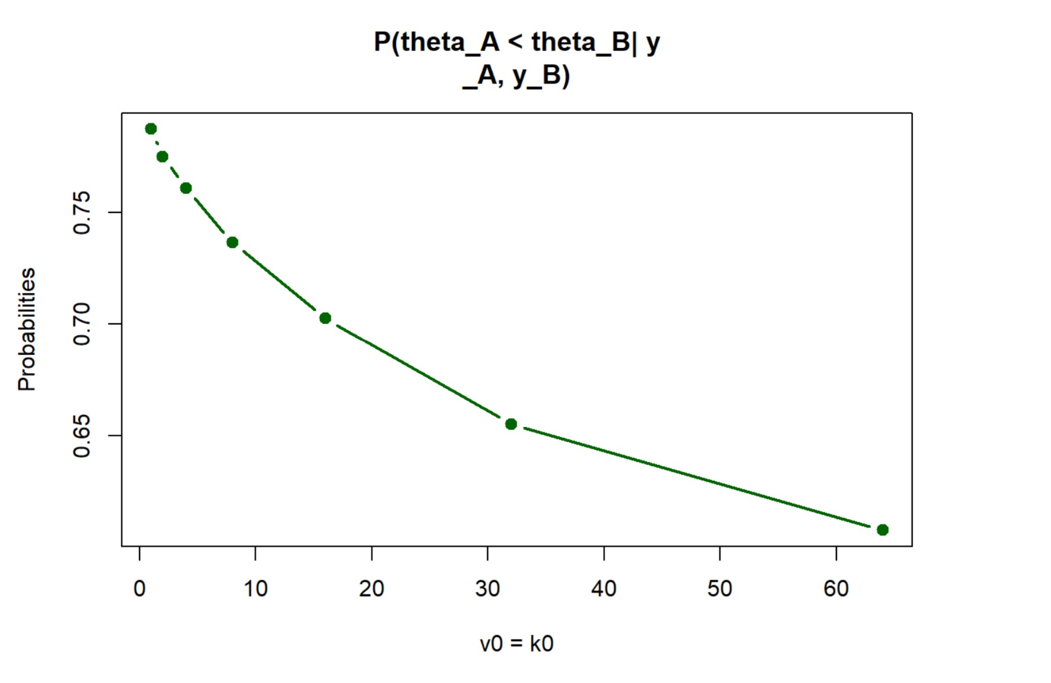
In a science classroom, 32 students were randomly assigned to two different study methods (A and B), with 16 students in each group. After several weeks of study, the students took a test designed to yield an average score of 75% with a standard deviation of 10. Group A scored an average of 75.2 with a standard deviation of 7.3, while Group B scored an average of 77.5 with a standard deviation of 8.1.
To evaluate the effectiveness of the study methods, we employed a conjugate normal prior with a mean
We utilized a Bayesian framework with Monte Carlo simulations to analyze the data and derive probabilities for the two study methods. The simulations allowed us to estimate the posterior distributions of the average scores for both methods and to calculate the probability that one method is better than the other.
The following parameters were set based on the problem statement:
- Sample size for each group: (n = 16)
- Average scores and standard deviations for groups A and B
- Prior parameters for Bayesian analysis
The simulation involved iterating through different prior sample sizes and computing the posterior distributions for both groups using Monte Carlo methods.
# Monte Carlo simulation for probabilities
probs <- c()
for (i in 1:length(k0)) {
  # Monte Carlo simulation for Group A
  mu_na <- (k0[i] * mu0 + n * ya) / (k0[i] + n)
  var_na <- 1 / (v0[i] + n) * (v0[i] * s20 + (n - 1) * sa^2 + (k0[i] * n) / (k0[i] + n) * (ya - mu0)^2)
  s_postsample_a <- sqrt(1 / rgamma(10000, (v0[i] + n) / 2, var_na * (v0[i] + n) / 2))
  theta_postsample_a <- rnorm(10000, mu_na, s_postsample_a / sqrt(k0[i] + n))

  # Monte Carlo simulation for Group B
  mu_nb <- (k0[i] * mu0 + n * yb) / (k0[i] + n)
  var_nb <- 1 / (v0[i] + n) * (v0[i] * s20 + (n - 1) * sb^2 + (k0[i] * n) / (k0[i] + n) * (yb - mu0)^2)
  s_postsample_b <- sqrt(1 / rgamma(10000, (v0[i] + n) / 2, var_nb * (v0[i] + n) / 2))
  theta_postsample_b <- rnorm(10000, mu_nb, s_postsample_b / sqrt(k0[i] + n))

  # Calculate probability that theta_A < theta_B
  mean_prob <- mean(theta_postsample_a < theta_postsample_b)
  probs <- c(probs, mean_prob)
}
The results were visualized in a plot displaying the relationship between the prior sample size
