NTHU_109062274_楊子慶 AIAS 2024 Lab 2 HW Submission

Gitlab code link

• Gitlab link: https://course.playlab.tw/git/eroiko/lab02

Environment setup

In this homework, I assume the gitlab repository will be cloned into ~/projects/lab02 folder inside acal-workspace-main container. I'd setup a bunch of scripts that helps us customize the container.

In lab02, there should exists a folder named general-scripts, please run the following commands before running homework program.

cd ~/projects/lab02
./general-scripts/setup_my_env.sh
./general-scripts/lab2-env.sh pip_install

All the programs and setup programs are well tested and can be run as soon as you follow this document.

:::danger NO additional packages and models needed to be installed as soon as you use the given setup scripts and programs I wrote step-by-step. :::

HW 2-1 Model Analysis Using Pytorch

How to run

cd ~/projects/lab02/hw2-1
python3 hw.py >> /dev/null

We'll see that several files are created in lab02/hw2-1, named w.r.t. each sub-homework.

> tree .
.
├── hw2-1-1-output.txt
├── hw2-1-2-output.txt
├── hw2-1-3-output.txt
├── hw2-1-4-output.txt
├── hw2-1-5-output.txt
├── hw.py
├── __pycache__
│   └── util.cpython-39.pyc
└── util.py

Program structure

I wrote a util.py module that collects some toolkit that will be frequently used in hw.py. This module will grow after each sub-homework.

The mostly used utility is perhaps the print_hw_result, printing the result to both console and well-named file in nice format.

def print_hw_result(mark: str, title: str, *lines: List[str]):
    """
    Print homework result and write corresponding file
    """
    def __print_to(file=None):
        print(f"[{mark}] {title}",
              *[f'\t{l}' for l in lines], sep="\n", end="\n\n", file=file)

    __print_to()
    with open(f"{os.path.dirname(script_dir)}/hw{mark}-output.txt", 'w') as f:
        __print_to(f)

To print result prettily, we usually collect things to be print into a list, unwrap and pass it to print_hw_result.

2-1-1. Calculate the number of model parameters

Code

device = "cuda" if torch.cuda.is_available() else "cpu"
device = torch.device(device)

# load GoogLeNet model
model = models.googlenet(weights=GoogLeNet_Weights.DEFAULT) \
              .to(device) \
              .eval() # locked as evaluation mode

input_shape = (3, 224, 224)

# 2-1-1 Calculate model parameters
total_params = sum(p.numel() for p in model.parameters())
trainable_params = sum(p.numel() for p in model.parameters() if p.requires_grad)
print_hw_result("2-1-1",
                "Calculate model parameters",
                f"Total parameters: {total_params}",
                f"trainable parameters: {trainable_params}",
                f"non-trainable parameters: {total_params - trainable_params}")

Note that install_dependency and print_hw_result are helper functions in util module.

Execution Result

[2-1-1] Calculate model parameters
	Total parameters: 6624904
	trainable parameters: 6624904
	non-trainable parameters: 0

2-1-2. Calculate memory requirements for storing the model weights.

Code

# 2-1-2 Calculate memory requirements for storing weights
total_param_bytes = sum(p.numel() * p.element_size() for p in model.parameters())
print_hw_result("2-1-2",
                "Calculate model memory requirements for storing weights",
                f"Total memory for parameters: {total_param_bytes} bytes")

Execution Result

[2-1-2] Calculate model memory requirements for storing weights
	Total memory for parameters: 26499616 bytes

2-1-3. Use Torchinfo to print model architecture including the number of parameters and the output activation size of each layer

Code

# 2-1-3. Use Torchinfo to print model architecture
#        including the number of parameters and
#        the output activation size of each layer
model_statistic = torchinfo.summary(model,
                                    input_shape,
                                    batch_dim=0,
                                    col_names=("num_params",
                                                "output_size",),
                                    verbose=0)
print_hw_result("2-1-3",
                "Peek model num_params and output size of each layer use Torchinfo",
                *str(model_statistic).split("\n"))

Execution Result

[2-1-3] Peek model num_params and output size of each layer use Torchinfo
	==========================================================================================
	Layer (type:depth-idx)                   Param #                   Output Shape
	==========================================================================================
	GoogLeNet                                --                        [1, 1000]
	├─BasicConv2d: 1-1                       --                        [1, 64, 112, 112]
	│    └─Conv2d: 2-1                       9,408                     [1, 64, 112, 112]
	│    └─BatchNorm2d: 2-2                  128                       [1, 64, 112, 112]
	├─MaxPool2d: 1-2                         --                        [1, 64, 56, 56]

        ...

	│    │    └─BasicConv2d: 3-70            55,552                    [1, 128, 7, 7]
	│    └─Sequential: 2-42                  --                        [1, 128, 7, 7]
	│    │    └─MaxPool2d: 3-71              --                        [1, 832, 7, 7]
	│    │    └─BasicConv2d: 3-72            106,752                   [1, 128, 7, 7]
	├─AdaptiveAvgPool2d: 1-17                --                        [1, 1024, 1, 1]
	├─Dropout: 1-18                          --                        [1, 1024]
	├─Linear: 1-19                           1,025,000                 [1, 1000]
	==========================================================================================
	Total params: 6,624,904
	Trainable params: 6,624,904
	Non-trainable params: 0
	Total mult-adds (G): 1.50
	==========================================================================================
	Input size (MB): 0.60
	Forward/backward pass size (MB): 51.63
	Params size (MB): 26.50
	Estimated Total Size (MB): 78.73
	==========================================================================================

2-1-4. Calculate computation requirements

Code

:::success Taking advantage of open source project https://github.com/sovrasov/flops-counter.pytorch.git, we can aquire macs of each kinds layer elegantly. :::

# install dependency
dep = ["ptflops"]
install_dependency(dep)

# ...

# 2-1-4. Calculate computation requirement
info_to_print = []

# Use open source project
#   https://github.com/sovrasov/flops-counter.pytorch.git
from ptflops import get_model_complexity_info

total_macs, _ = get_model_complexity_info(model,
                                          input_shape,
                                          output_precision=10,
                                          print_per_layer_stat=False,
                                          ignore_modules=[torch.nn.Dropout,],)

info_to_print.append(f"Total MACs is {total_macs}")

def get_children(m) -> List[Union[List, str]]:
    """
    Get listed layers of a pytorch model
    """
    if next(m.children(), None) == None:
        return m.__class__
    else:
        return [get_children(c) for c in m.children()]

layers = { *flatten(get_children(model)) }

# the default macs exists when we ignore all possible layers,
#   which we're not curious about, so we should record it
#   and subtract it out for all results.
default_layer_macs, _ = get_model_complexity_info(model,
                                               input_shape,
                                               output_precision=10,
                                               ignore_modules=[*layers],
                                               as_strings=False,
                                               print_per_layer_stat=False,)
layers = layers - { torch.nn.Dropout }
# iterate sorted set to ensure that anytime the result order is the same
for layer in sorted(layers, key=lambda e: e.__name__):
    layer_macs, _ = get_model_complexity_info(model,
                                              input_shape,
                                              output_precision=10,
                                              ignore_modules=[*(layers-{layer})],
                                              as_strings=False,
                                              print_per_layer_stat=False,)
    layer_macs -= default_layer_macs
    info_to_print.append(f"MACs for [ {layer.__name__:^17} ] layers is {layer_macs:>11}")
print_hw_result("2-1-4",
                "Calculate computation requirements",
                *info_to_print)

Execution Result

:::success Note: This shows macs of all kinds of layers, satisfying bonus requirement. :::

[2-1-4] Calculate computation requirements
	Total MACs is 1.513907448 GMac
	MACs for [ AdaptiveAvgPool2d ] layers is       50176
	MACs for [    BatchNorm2d    ] layers is     6452320
	MACs for [      Conv2d       ] layers is  1497352192
	MACs for [      Linear       ] layers is     1025000
	MACs for [     MaxPool2d     ] layers is     2875712

2-1-5. Use forward hooks to extract the output activations of the Conv2d layers.

Code

:::info You can configurate forward_input_for_2_1_5 and torch.set_printoptions with reasonable value.

This method of implementation is simply to add fetch_output_activations forward hook, and add_unique_name forward pre-hook to identify each Conv2d layer. :::

#! 2-1-5 configurable variable
#! forward_input_for_2_1_5 is variable that with forward to model
forward_input_for_2_1_5 = torch.zeros(1, *input_shape)
forward_input_for_2_1_5 = forward_input_for_2_1_5.to(device)
torch.set_printoptions(edgeitems=1) # print less info for output readibility

# ...

# 2-1-5 Use forward hooks to extract the output activations of the Conv2d layers
info_to_print = []
conv2d_count = 0
focus_layer_name = "Conv2d"

def add_unique_name(module: torch.nn.Module, _, __):
    global conv2d_count
    for m in module.modules():
        if not hasattr(m, 'my_name') and m.__class__.__name__ == focus_layer_name:
            m.my_name = f"{focus_layer_name}-No.{conv2d_count}"
            conv2d_count += 1

def fetch_output_activations(module: torch.nn.Module, _, output: torch.Tensor):
    if focus_layer_name == module.__class__.__name__:
        formatted_str = '\n\t\t'.join(str(output).split('\n'))
        info_to_print.append(f"Module [ {module.my_name:^12} ] has output activation:\n\t\t{formatted_str}\n")

model.apply(lambda m: m.register_forward_hook(add_unique_name) and
            m.register_forward_hook(fetch_output_activations))
model(forward_input_for_2_1_5)
print_hw_result("2-1-5",
                "Use forward hooks to extract the output activations of the Conv2d layers",
                *info_to_print)

Execution Result

[2-1-5] Use forward hooks to extract the output activations of the Conv2d layers
	Module [ Conv2d-No.0  ] has output activation:
		tensor([[[[ 0.1498,  ..., -0.2169],
		          ...,
		          [-0.1768,  ..., -0.2147]],

		         ...,

		         [[-0.1682,  ...,  0.0211],
		          ...,
		          [ 0.0252,  ...,  0.2535]]]], device='cuda:0',
		       grad_fn=<ConvolutionBackward0>)

	Module [ Conv2d-No.1  ] has output activation:
		tensor([[[[-2.5879,  ..., -2.4359],
		          ...,
		          [-2.4752,  ..., -2.3224]],

		         ...,

		         [[-3.1649,  ..., -3.1641],
		          ...,
		          [-3.1283,  ..., -3.0907]]]], device='cuda:0',
		       grad_fn=<ConvolutionBackward0>)

	...

	Module [ Conv2d-No.56 ] has output activation:
		tensor([[[[ 0.0731,  ..., -0.1592],
		          ...,
		          [-0.2058,  ...,  0.0958]],

		         ...,

		         [[ 0.3016,  ..., -0.1947],
		          ...,
		          [ 0.1403,  ..., -0.2072]]]], device='cuda:0',
		       grad_fn=<ConvolutionBackward0>)

HW 2-2 Add more statistics to analyze the an ONNX model Using sclblonnx

How to run

cd ~/projects/lab02/hw2-2
python3 hw.py >> /dev/null

We'll see that several files are created in lab02/hw2-2, named w.r.t. each sub-homework.

> tree .
.
├── hw2-2-1-output.txt
├── hw2-2-{2_3}-output.txt
├── hw.py
├── models
│   └── model.onnx
├── onnx_helper.py
├── __pycache__
│   ├── ...
└── util.py

Program structure

Beside util, I add onnx_helper module that collects some toolkit that helps us inspect an arbitrary ONNX model, also reusing and expanding it in hw2-3.

In hw.py, you'll see that...

from util import *

model_path_prefix = "models"
model_path = f"{model_path_prefix}/model.onnx"
if not os.path.exists(model_path):
    if not os.path.exists(model_path_prefix):
        run_process(["mkdir", "-p", model_path_prefix])
    download_file("https://github.com/onnx/models/raw/main/validated/vision/classification/mobilenet/model/mobilenetv2-10.onnx",
                  model_path)
else:
    print(f"Model {model_path} exist, skip downloading")

Taking the advantage of my util module, we install the required model from https://github.com/onnx/models/raw/main/validated/vision/classification/mobilenet/model/mobilenetv2-10.onnx if it does not exists, putting it in the right place we're going to use.

2-2-1. model characteristics

Code

In hw.py, the main script, you'll see the lines which is simple enough to understand without verbose comments.

# 2-2-1 Model characteristics
import onnx
from onnx_helper import OnnxHelper

model = onnx.load(model_path)
helper = OnnxHelper(model)

unique_ops = { node.op_type for node in model.graph.node }
model_op_list = []

info_list = [
    "Unique operators:",
    # use sorted to make sure result is consistent anytime
    "\t" + "\n\t\t".join(sorted(unique_ops)),
    "",
    "Attribute range of all the operators:",
    *json_stringify({ "GoogleNet": helper.summary() }, indent=1),
]
print_hw_result("2-2-1",
                "Model characteristics",
                *info_list)

Of course, OnnxHelper::summary method is the one that actually deal with fetching ONNX model summary in onnx_helper.py.

class OnnxHelper:
    def summary(self, wrap_graph_name = False, verbose = False) -> list[str]:
        json = []
        graph = self.model.graph
        for n in graph.node:
            data_val = {}
            # fetch input info if exist
            if len(n.input) > 0:
                input_info = {}
                for i_node in n.input:
                    try:
                        p = self.fetch_proto(i_node)
                        sz = self.fetch_size(p)
                        input_info[p.name] = sz
                    except ValueError as e:
                        print(e)
                data_val["input"] = input_info
            # fetch output info if exist
            if len(n.output) > 0:
                output_info = {}
                for o_node in n.output:
                    try:
                        p = self.fetch_proto(o_node)
                        sz = self.fetch_size(p)
                        output_info[p.name] = sz
                    except ValueError as e:
                        print(e)
                data_val["output"] = output_info
            # fetch attribute
            attr_val = self.fetch_attr(n)
            if len(attr_val) > 0:
                data_val["attribute"] = attr_val
            json.append({ n.op_type: data_val })

        if wrap_graph_name:
            json = { self.model.graph.name: json }

        if verbose:
            print("\n".join(json_stringify(json)))

        return json

Since OnnxHelper is a well designed object, I should not paste all the methods here that disturbing us to understand the main logic.

The code can be splitted into 3 parts for each iteration of model node: fetching input, output and attribute. After each iteration, we collect the result onto json with json format that can be recognized, parsed and printed elegantly by util functions.

The other methods are documented and well type-marked so we can understand them without looking the implementation.

class OnnxHelper:
    def fetch_proto(self, fid: str):
        """
        Fetch `ValueInfoProto` or `TensorProto` using field identifier `fid`
        """

    def fetch_size(_, proto: Union[onnx.ValueInfoProto, onnx.TensorProto]) -> \
        dict[Union[Literal["shape"],
                   Literal["memory_size"]],
             int]:
        """
        Fetch shape and memory usage information w.r.t. given `proto`

        Returns dict form of `{ "shape", "memory_size" }`, \
            unit of `memory_size` is byte
        """

    def fetch_attr(_, node: onnx_ml_pb2.NodeProto) -> dict:
        """
        Get attributes from a onnx node proto as `dict`
        """

:::success Note: The implementation of fetch_attr is kind of tricky that parsing the output of AttributeProto::ListFields to get all the attributes according to attribute format (a single value or a tensor). :::

Execution Result

[2-2-1] Model characteristics
	Unique operators:
		Add
		Clip
		Concat
		Constant
		Conv
		Gather
		Gemm
		GlobalAveragePool
		Reshape
		Shape
		Unsqueeze

	Attribute range of all the operators:
		GoogleNet
			Conv
				input
					input
						shape       : (0, 3, 224, 224)
						memory_size : 602112
					475
						shape       : (32, 3, 3, 3)
						memory_size : 3456
					476
						shape       : (32,)
						memory_size : 128
				output
					474
						shape       : (0, 32, 112, 112)
						memory_size : 1605632
				attribute
					dilations    : [1, 1]
					group        : 1
					kernel_shape : [3, 3]
					pads         : [1, 1, 1, 1]
					strides      : [2, 2]
			Clip
				input
					474
						shape       : (0, 32, 112, 112)
						memory_size : 1605632
				output
					317
						shape       : (0, 32, 112, 112)
						memory_size : 1605632
				attribute
					max : 6.0
					min : 0.0
			Conv
				input
					317
						shape       : (0, 32, 112, 112)
						memory_size : 1605632
					478
						shape       : (32, 1, 3, 3)
						memory_size : 1152
					479
						shape       : (32,)
						memory_size : 128
				output
					477
						shape       : (0, 32, 112, 112)
						memory_size : 1605632
				attribute
					dilations    : [1, 1]
					group        : 32
					kernel_shape : [3, 3]
					pads         : [1, 1, 1, 1]
					strides      : [1, 1]

                        ...

			Reshape
				input
					464
						shape       : (0, 1280, 1, 1)
						memory_size : 5120
					471
						shape       : (2,)
						memory_size : 16
				output
					472
						shape       : ()
						memory_size : 0
			Gemm
				input
					472
						shape       : ()
						memory_size : 0
					classifier.1.weight
						shape       : (1000, 1280)
						memory_size : 5120000
					classifier.1.bias
						shape       : (1000,)
						memory_size : 4000
				output
					output
						shape       : (0, 1000)
						memory_size : 4000
				attribute
					alpha  : 1.0
					beta   : 1.0
					transB : 1

2-2-{2, 3}. {Data bandwidth, activation memory storage} requirement

Code

:::info Note:

bw stands for bandwidth. tot stands for total. i stands for input. o stands for output.

Formulas:

• Data bandwidth: peek activation bandwidth $$ \max({\rm{Output\ memory\ usages}}) $$
• Activation memory storage: total activation bandwidth, i.e. $$ \sum^{layer}_{i}{\rm{Output\ memory\ usage}_i} $$
• (Addition) Total memory storage $$ \rm{Input\ memory\ usage} + \sum^{layer}_{i}{\rm{Output\ memory\ usage}_i} $$ :::

# 2-2-{2,3} Bandwidth requirement
bw_ls = [] # memory bandwidth list
max_bw = 0
tot_bw, tot_i_bw, tot_o_bw = 0, 0, 0
i_bw, o_bw = 0, 0 # input and output bandwidth

for cnt, n in enumerate(model.graph.node):
    i_bw, o_bw = 0, 0 # initialize io bw
    if len(n.input) > 0:
        sz = helper.fetch_size(helper.fetch_proto(n.input[0]))
        i_bw += sz["memory_size"]
    if len(n.output) > 0:
        sz = helper.fetch_size(helper.fetch_proto(n.output[0]))
        o_bw += sz["memory_size"]
    if cnt == 0: # only reserve first input size to total bandwidth
        tot_bw += i_bw
    max_bw = max(max_bw, i_bw + o_bw)
    tot_bw += o_bw
    tot_i_bw += i_bw
    tot_o_bw += o_bw
    bw_ls.append([n.name, i_bw, o_bw, i_bw + o_bw])
bw_ls.append([*["-----"] * 4]) # splitter of table
bw_ls.append(["Total I/O activation", tot_i_bw, tot_o_bw, "-"])

info_list = [
    f"Peek bandwidth (2-2-2): {max_bw} bytes",
    f"Total activation bandwidth (2-2-3): {tot_o_bw} bytes",
    f"Total bandwidth: {tot_bw} bytes\n",
    "List of bandwidth of each layer:\n",
    *tabulate(bw_ls,
              tablefmt="rounded_outline",
              colalign=["left", *(["right"] * 3)],
              headers=["layer",
                       "input bw",
                       "output bw",
                       "bandwidth"]).split("\n"),
]

print_hw_result("2-2-{2_3}",
                "Bandwidth requirement",
                *info_list)

Execution Result

:::info Note: Table List of bandwidth of each layer is for inspecting the bandwidth of each layers. :::

[2-2-{2_3}] Bandwidth requirement
	Peek bandwidth (2-2-2): 9633792 bytes
	Total activation bandwidth (2-2-3): 52010328 bytes
	Total bandwidth: 52612440 bytes

	List of bandwidth of each layer:

	╭──────────────────────┬────────────┬─────────────┬─────────────╮
	│ layer                │   input bw │   output bw │   bandwidth │
	├──────────────────────┼────────────┼─────────────┼─────────────┤
	│ Conv_0               │     602112 │     1605632 │     2207744 │
	│ Clip_1               │    1605632 │     1605632 │     3211264 │
	│ Conv_2               │    1605632 │     1605632 │     3211264 │
        ...
	│ Shape_98             │     250880 │          32 │      250912 │
	│ Constant_99          │          0 │           0 │           0 │
	│ Gather_100           │         32 │           0 │          32 │
	│ Unsqueeze_101        │          0 │           8 │           8 │
	│ Concat_102           │          8 │          16 │          24 │
	│ Reshape_103          │       5120 │           0 │        5120 │
	│ Gemm_104             │          0 │        4000 │        4000 │
	│ -----                │      ----- │       ----- │       ----- │
	│ Total I/O activation │   52859304 │    52010328 │           - │
	╰──────────────────────┴────────────┴─────────────┴─────────────╯

HW 2-3 Build tool scripts to manipulate an ONNX model graph

How to run

cd ~/projects/lab02/hw2-3
python3 hw.py >> /dev/null

We'll see that several files are created in lab02/hw2-3, named w.r.t. each sub-homework.

> tree .
.
├── dynamic_linear.py
├── hw2-3-0-output.txt
├── hw2-3-1-output.txt
├── hw2-3-2-output.txt
├── hw2-3-3-output.txt
├── hw2-3-4-output.txt
├── hw.py
├── models
│   ├── model.onnx
│   ├── modified.onnx
│   ├── subgraph1.onnx
│   └── subgraph2.onnx
├── onnx_helper.py
├── __pycache__
│   ├── ...
└── util.py

General settings

The question is say that assuming we're using some hardware which can at most calculating GEMM with some limited M, N, K value.

In hw.py, we can set them by changing these variables:

# max width of each dimension
m_mx, n_mx, k_mx = 64, 64, 64

As code shown above, the given default configuration matches the description of HW 2-3.

2-3-1. create a subgraph (1) that consist of a single Linear layer of size MxKxN

Code

In 2-3-{1, 2}, we can configure M, K, N of an arbitrary GEMM operation by changing the line below.

# 2-3-1 + 2-3-2
m, k, n = 32, 64, 128

We'll using those configurations to construct a DynamicLinear object I designed that creates both test_model member for testing (i.e. subgraph1) and model member as real DynamicLinear (i.e. subgraph2).

my_model = DynamicLinear(m,
                         k,
                         n,
                         m_mx,
                         k_mx,
                         n_mx,
                         GemmInputInfo("A"),
                         GemmInputInfo("B"),
                         GemmInputInfo("bias"),
                         GemmOutputInfo("C")
                         )

# 2-3-1
test_model_path = f"{model_dir}/subgraph1.onnx"
onnx.save(my_model.test_model, test_model_path)
test_helper = OnnxHelper(my_model.test_model, to_check=True)
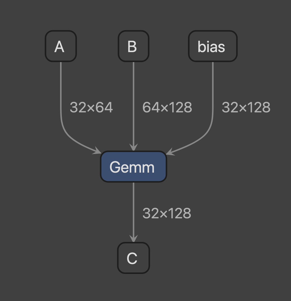
print_hw_result("2-3-1",
                "Create a subgraph (1) that consist of a single Linear layer of size MxKxN",
                *json_stringify(test_helper.summary(wrap_graph_name=True, override_name="Subgraph 1")))

So the point is how we create test_model member in this part.

from util import *
import numpy as np
import onnx
from onnx import TensorProto, helper, checker
from onnx.reference import ReferenceEvaluator

...

class DynamicLinear:
    def initialize_test_graph(self):
        """
        Initialize graph and model equivalent to those of DynamicLinear for testing
        """
        ((a_name, trans_a, a_shape),
         (b_name, trans_b, b_shape), bias_name), c_name = self.get_io_info()

        a_name = self.name_it(a_name, True)
        b_name = self.name_it(b_name, True)
        bias_name = self.name_it(bias_name, True)
        c_name = self.name_it(c_name, True)

        self.test_graph = helper.make_graph(nodes=[helper.make_node("Gemm",
                                                                    inputs=(a_name, b_name, bias_name),
                                                                    outputs=(c_name,),
                                                                    transA=trans_a,
                                                                    transB=trans_b,
                                                                    ),],
                                            name=f"TestGraph_{self.name}",
                                            inputs=[helper.make_tensor_value_info(a_name,
                                                                                  TensorProto.FLOAT,
                                                                                  a_shape),
                                                    helper.make_tensor_value_info(b_name,
                                                                                  TensorProto.FLOAT,
                                                                                  b_shape),
                                                    helper.make_tensor_value_info(bias_name,
                                                                                  TensorProto.FLOAT,
                                                                                  (self.m, self.n))],
                                            outputs=[helper.make_tensor_value_info(c_name,
                                                                                   TensorProto.FLOAT,
                                                                                   (self.m, self.n))],)
        self.test_model = helper.make_model(self.test_graph)

We can see that the implementation is quite simple, according to ONNX official documentation, we can reference the GEMM operator and use it with correct arguments.

Visualize the subgraph (1)

Before looking at visualized graph, we can reuse our OnnxHelper::summary method to peek it in plain text format:

[2-3-1] Create a subgraph (1) that consist of a single Linear layer of size MxKxN
	Subgraph 1
		Gemm
			input
				A
					shape       : (32, 64)
					memory_size : 8192
				B
					shape       : (64, 128)
					memory_size : 32768
				bias
					shape       : (32, 128)
					memory_size : 16384
			output
				C
					shape       : (32, 128)
					memory_size : 16384
			attribute
				transA : 0
				transB : 0

Then, use the follow command to visualize test model by netron.

python3 -c "import netron; netron.start('./models/subgraph1.onnx', 10000)"

You'll see a graph like this:

2-3-2. create a subgraph (2) as shown in the above diagram for the subgraph (1)

Code

Continued with 2-3-1, we can access model member to get subgraph2.

# 2-3-2
dl_model_path = f"{model_dir}/subgraph2.onnx"
onnx.save(my_model.model, dl_model_path)
dl_helper = OnnxHelper(my_model.model)
print_hw_result("2-3-2",
                "Create a subgraph (2) as shown in the above diagram for the subgraph (1)",
                *json_stringify(dl_helper.summary(wrap_graph_name=True, override_name="Subgraph 2")))

The implementation of DynamicLinear layer is fully parameterized In initialize_graph method, I generalize the split, calculate and concat process with a Normal Matrix Multiplication process. That is, we don't need to care the size to be split, we just treat the operands as many matrix-elements that're ready to join a normal matrix multiplication process, i.e. the implementation will be like something like what I commented for initialize_graph method:

def initialize_graph(self):
    """
    Create a Linear graph with generalization of all dimension factors

    The implementation simulates the code snippet below,
    i.e. Matrix multiplication

    ```python
    c_on_m_axis = []
    for _m in range(m_factor):
        c_on_n_axis = [0] * n_factor
        for _n in range(n_factor):
            mm_list = []
            for _k in range(k_factor):
                mm_list.append(a_splits[_k][_m] * b_splits[_n][_k])
            c_on_n_axis[_n] = sum(mm_list)
        c_list = concat(c_on_n_axis)
    c = concat(c_on_m_axis)
    ```
    """

Undoutedly, the real implementation is quite more complicated. First, the X_factor indicates how many number along X side should be split. For example, if m is 128 and mx_m (max size along m axis) is 64, then m_factor will be $\dfrac{m}{mx} = 2$. To deal with indivisible cases, we should round up for the remainders joining the following process, also we may need to know whether the factor of some side is divisible, that's what DynamicLinear::get_factor method does.

class DynamicLinear:
    ...
    def get_factor(side: int, max_side: int) -> tuple[int, bool]:
        """
        helper function to get splitting factor for some dimension
        return (factor, integer-divisible)
        """
        factor = side // max_side
        complement = 0 if side % max_side == 0 else 1

        return (factor + complement if factor != 0 else 1, complement == 0)
    ...
    def initialize_graph(self):
        ...
        # define factors
        m_factor, m_is_div = DynamicLinear.get_factor(m, m_mx)
        k_factor, k_is_div = DynamicLinear.get_factor(k, k_mx)
        n_factor, n_is_div = DynamicLinear.get_factor(n, n_mx)

Before doing multiplication, we should quantize the two input matrices. But before we jump in to split inputs, we should first know how to build a operator node. They're combined with three objects:

1. Name: str
2. Value information: ValueInfoProto, can be generated using onnx::helper::make_tensor_value_info
3. Node: NodeProto, can be generated using onnx::helper::make_node

For readibility, in the implementation, I always write them with the following coding style.

# COMMENT of some node
#   First, define inner output tensor of split result
name_or_name_list = ... # str or List[str]
#   Second, define tensor info...
name_or_name_list_tensor = ... # use helper.make_tensor_value_info
#   Preparation complete, create ...
name_or_name_list_layer = ... # use helper.make_node
self.check_node(name_or_name_list_layer) # check whether layer is valid

After generating the layers with in each contains three objects, we can pass them and form a model graph ad below:

self.inputs = [a_node, b_node, bias_node]
self.outputs = [output_node]
self.nodes = ... # [layers]
self.value_info = ... # [tensors]
self.initializer = ... # [tensors], additional tensor information that is used in generating node

self.graph = helper.make_graph(nodes=self.nodes,
                               name=f"DynamicLinear_{self.name}",
                               inputs=self.inputs,
                               outputs=self.outputs,
                               value_info=self.value_info,
                               initializer=self.initializer)

Now, we're ready to introduce the implementation! The whole process is pipelined as:

1. Check if we need to add additional transpose layer according to input X_info: for X in a, b
2. Split along the first dimension: X_Y_splits (Y as the first dimension of X)
3. Split along the second dimension: X_splits, so we finish quantizing the inputs.
4. Do element-wise multiplication along k side with MatMul: mms
5. Sum up the result of element-wise multiplication: sums
6. Concatenate along the second dimension n: concat_ns
7. Concatenate along the first dimension m: concat_m
8. Add the result and bias input: addition_layer
9. Add additional transpose layer on the front if needed according to the result of the first step

For example, the code below shows how I implement the forth mms part:

# MatMul: equivalent to k-level for loop of matrix multiplication
#   a_splits and b_splits are the input of this layer
#
#   First define name of inner output with radix (m, n, k)
#       notice that radix like (m, n, k) should change its mark like a counter
mms = [[[self.name_it(f"MatMul_m{_m}_n{_n}_k{_k}")
         for _m in range(m_factor)]
        for _n in range(n_factor)]
       for _k in range(k_factor)]
#   Second, define inner output of general matrix multiplication result
mm_tensors = [[[helper.make_tensor_value_info(mms[_k][_n][_m],
                                              TensorProto.FLOAT,
                                              (m_cnt, n_cnt))
                for _m, m_cnt in enumerate(m_slice_list)]
               for _n, n_cnt in enumerate(n_slice_list)]
              for _k in range(k_factor)]
#   Preparation complete, create MatMul layers
mm_layers = [[[helper.make_node("MatMul",
                                inputs=[a_splits[_k][_m], b_splits[_n][_k]],
                                outputs=[mms[_k][_n][_m]],
                                name=mms[_k][_n][_m])
               for _m in range(m_factor)]
              for _n in range(n_factor)]
             for _k in range(k_factor)]

Now we know how we can fully parameterize DynamicLinear layer if we follow the pipeline instruction.

Visualize the subgraph (2)

Before looking at visualized graph, we can reuse our OnnxHelper::summary method to peek it in plain text format:

:::info Below result is when (M, K, N) = (32, 64, 128). :::

[2-3-2] Create a subgraph (2) as shown in the above diagram for the subgraph (1)
	Subgraph 2
		Split
			input
				A
					shape       : (32, 64)
					memory_size : 8192
				dl_m_slices
					shape       : (1,)
					memory_size : 8
			output
				dl_A_Split_m0
					shape       : (32, 64)
					memory_size : 8192
			attribute
				axis : 0
		Split
			input
				B
					shape       : (64, 128)
					memory_size : 32768
				dl_k_slices
					shape       : (1,)
					memory_size : 8
			output
				dl_B_Split_k0
					shape       : (64, 128)
					memory_size : 32768
			attribute
				axis : 0

                ...
		Add
			input
				dl_Concat_M
					shape       : (32, 128)
					memory_size : 16384
				bias
					shape       : (32, 128)
					memory_size : 16384
			output
				C
					shape       : (32, 128)
					memory_size : 16384

Then, use the follow command to visualize test model by netron.

python3 -c "import netron; netron.start('./models/subgraph2.onnx', 10000)"

You'll see a graph like this:

(M, K, N)	(32, 64, 128)	(128, 128, 128)
example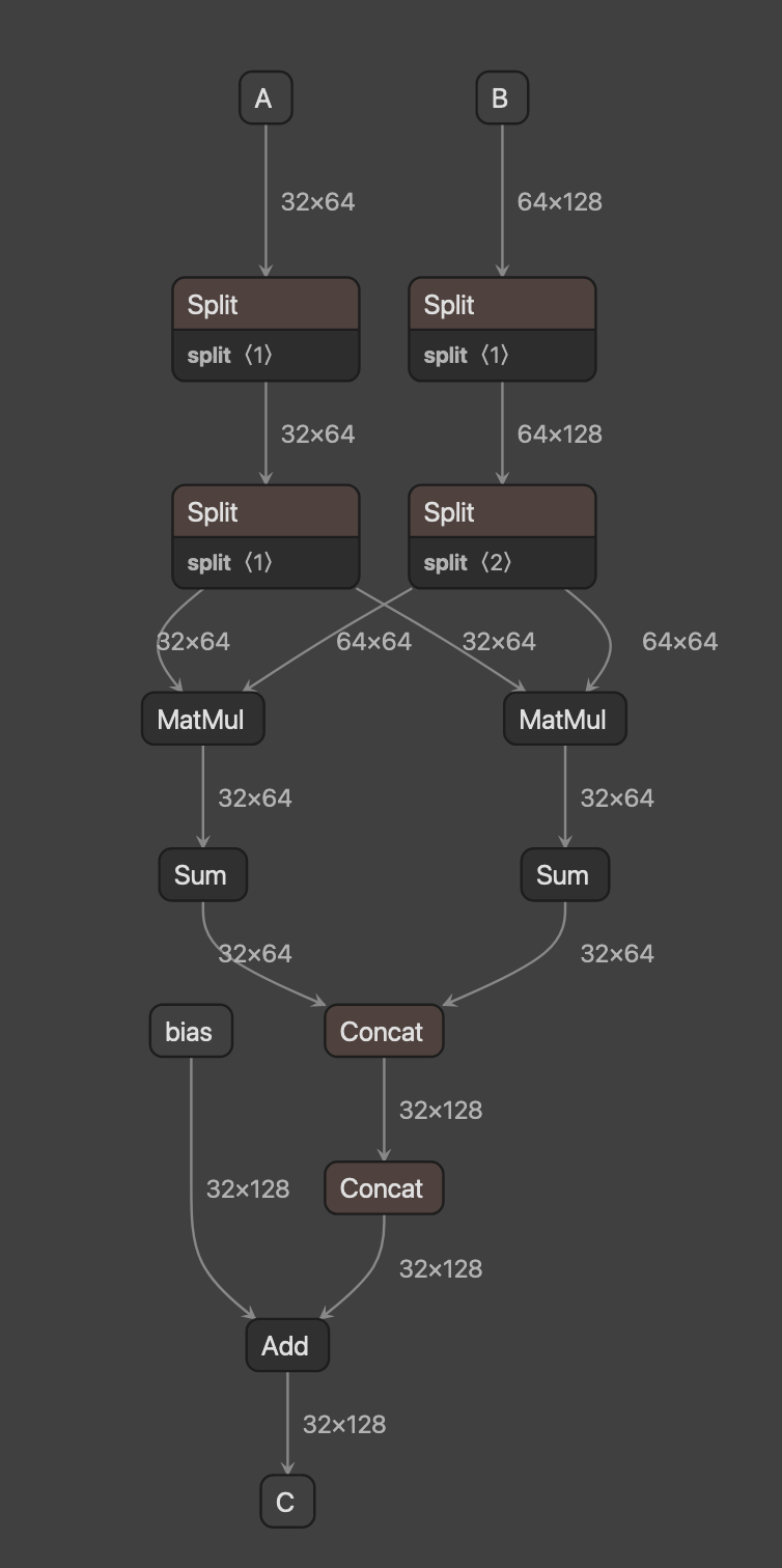

2-3-3. replace the Linear layers in the AlexNet with the equivalent subgraphs (2)

Code

Before replacing Alexnet, we should first make one in onnx format as the following code does.

# 2-3-3
# fetch alexnet model
from torchvision import models
import torch

alexnet_model_path = f"{model_dir}/model.onnx"
# alexnet_model_url = "https://github.com/onnx/models/raw/main/validated/vision/classification/alexnet/model/bvlcalexnet-12.onnx"
if not os.path.exists(alexnet_model_path):
    if not os.path.exists(model_dir):
        run_process(["mkdir", "-p", model_dir])

    device = "cuda" if torch.cuda.is_available() else "cpu"
    device = torch.device(device)

    # Download alexnet from torchvision, convert to ONNX model and save it
    #   ref: https://pytorch.org/docs/stable/onnx_torchscript.html
    dummy_input = torch.randn(1, 3, 224, 224, device=device)
    alexnet_model = models.alexnet().to(device)
    alexnet_model.eval() # Model must be in evaluation mode for export

    # Providing input and output names sets the display names for values
    # within the model's graph. Setting these does not change the semantics
    # of the graph; it is only for readability.
    #
    # The inputs to the network consist of the flat list of inputs (i.e.
    # the values you would pass to the forward() method) followed by the
    # flat list of parameters. You can partially specify names, i.e. provide
    # a list here shorter than the number of inputs to the model, and we will
    # only set that subset of names, starting from the beginning.
    input_names = [ "actual_input_1" ] + [ "learned_%d" % i for i in range(16) ]
    output_names = [ "output1" ]

    torch.onnx.export(alexnet_model,
                    dummy_input,
                    alexnet_model_path,
                    verbose=True,
                    input_names=input_names,
                    output_names=output_names)
else:
    print(f"Model {alexnet_model_path} exist, skip downloading")

# Alexnet: load and initialize helper
alexnet_model = onnx.load(alexnet_model_path)
alexnet_helper = OnnxHelper(alexnet_model, to_check=True)
print_hw_result("2-3-0",
                "Peek converted Alexnet",
                *json_stringify(alexnet_helper.summary(wrap_graph_name=True, override_name="Alexnet")))

# Alexnet (to be modified): load and initialize helper
my_alexnet_model = onnx.load(alexnet_model_path)
my_alexnet_helper = OnnxHelper(my_alexnet_model, to_check=True)

Now we have alexnet prepared, let's replace all the GEMM layers into our DynamicLinear layers.

def parse_gemm_size(info: dict[OnnxHelper.NodeInfoType, dict]) \
    -> tuple[tuple[tuple[str, ],
                   tuple[str, ],
                   tuple[str, ],
                   tuple[str, ]],
             tuple[bool, bool],
             tuple[int, int, int]]:
    """
    Parse and return m, k, n in Gemm operation
    """
    ...


# Manipulate onnx model using OnnxHelper API implement by myself
replacements: List[tuple[int, onnx.GraphProto]] = []
my_models: List[DynamicLinear] = []
# Prepare replacement layers
for idx in alexnet_helper.select_all(lambda n: n.op_type == "Gemm"):
    _, node_info = alexnet_helper.get_info_from_node(idx)
    (A, B, bias, C), (trans_a, trans_b), (m, k, n) = parse_gemm_size(node_info)

    a_name, b_name, bias_name, c_name = A[0], B[0], bias[0], C[0]

    model = DynamicLinear(m,
                          k,
                          n,
                          m_mx,
                          k_mx,
                          n_mx,
                          a_info=GemmInputInfo(a_name, trans_a),
                          b_info=GemmInputInfo(b_name, trans_b),
                          bias_info=GemmInputInfo(bias_name),
                          c_info=GemmOutputInfo(c_name),
                          name=str(idx),
                          named_ls=my_alexnet_helper.get_named_list()
                          )

    # this is for sure that my model works gracefully
    model_helper = OnnxHelper(model.model)

    replacements.append((idx, model.graph))
    my_models.append(model)

# Replace all GEMM layers at correct place
my_alexnet_helper.replace_all(replacements)
onnx.save(my_alexnet_helper.model, f"{model_dir}/modified.onnx") # for viewing result

print_hw_result("2-3-3",
                "Replace the Linear layers in the AlexNet with the equivalent subgraphs (2)",
                *json_stringify(my_alexnet_helper.summary(wrap_graph_name=True)))

We can see how OnnxHelper::replace_all manipulate the graph:

def replace_all(self, replacements: List[tuple[int, onnx_ml_pb2.GraphProto]]):
    """
    Replace all the nodes w.r.t. given node indices and re-indexing.
    replacements: list of `<< old_node_idx, new_graph >>` pair
    """
    replacements.sort(key = lambda idx: -idx[0])

    this_graph = self.model.graph
    for node_idx, replacement in replacements:
        popped_node = this_graph.node.pop(node_idx)
        for n in reversed(replacement.node):
            this_graph.node.insert(node_idx, n)
        this_graph.value_info.extend(replacement.value_info)
        this_graph.initializer.extend(replacement.initializer)

    self.to_check = True
    self.indexing()

The trick is to replace nodes from bigger index to smaller one, assuring the correct order of node, value_info and initializer of result while extending them.

The DynamicLinear::indexing is to rebuild members holding correct additional information extracted from model graph.

Visualize the transformed model graph

Before looking at visualized graph, we can reuse our OnnxHelper::summary method to peek it in plain text format:

[2-3-3] Replace the Linear layers in the AlexNet with the equivalent subgraphs (2)
	main_graph
		Conv
			input
				actual_input_1
					shape       : (1, 3, 224, 224)
					memory_size : 602112
				learned_0
					shape       : (64, 3, 11, 11)
					memory_size : 92928
				learned_1
					shape       : (64,)
					memory_size : 256
			output
				/features/features.0/Conv_output_0
					shape       : (1, 64, 55, 55)
					memory_size : 774400
			attribute
				dilations    : [1, 1]
				group        : 1
				kernel_shape : [11, 11]
				pads         : [2, 2, 2, 2]
				strides      : [4, 4]
		Relu
			input
				/features/features.0/Conv_output_0
					shape       : (1, 64, 55, 55)
					memory_size : 774400
			output
				/features/features.1/Relu_output_0
					shape       : (1, 64, 55, 55)
					memory_size : 774400
                ...
				dl_19_Sum_m0_n13
					shape       : (1, 64)
					memory_size : 256
				dl_19_Sum_m0_n14
					shape       : (1, 64)
					memory_size : 256
				dl_19_Sum_m0_n15
					shape       : (1, 40)
					memory_size : 160
			output
				dl_19_Concat_m0
					shape       : (1, 1000)
					memory_size : 4000
			attribute
				axis : 1
		Concat
			input
				dl_19_Concat_m0
					shape       : (1, 1000)
					memory_size : 4000
			output
				dl_19_Concat_M
					shape       : (1, 1000)
					memory_size : 4000
			attribute
				axis : 0
		Add
			input
				dl_19_Concat_M
					shape       : (1, 1000)
					memory_size : 4000
				learned_15
					shape       : (1000,)
					memory_size : 4000
			output
				output1
					shape       : (1, 1000)
					memory_size : 4000

Then, use the follow command to visualize test model by netron.

python3 -c "import netron; netron.start('./models/modified.onnx', 10000)"

You'll see a graph like this:

:::danger Yes, you just saw I put an image of a single white line. If you zoom in crazily, you should see something like...

We'll find out that it is too difficult to see the visualized graph. Although we can see that three gemm layers are replaced by DynamicLinear graph, they're too wide to be displayed...

I would say that the plain-text version may be an expedient way to peek the structure of graph. :::

2-3-4. Correctness Verification

Code

Before jumping into the implementation, we should first understand and trust that onnx operators used in DynamicLinear are memorylessness, that is, given the same inputs, the function always output the same output.

So rather than compare the whole modified alexnet model with the original one consuming lots of time and effort, if we TRUST the memorylessness of the implementation of onnx, we can just test the replaced part, i.e. compare model member and test_model member. That's how the test_equivalence method works.

Since we'd modified three alexnet GEMM operators, we can collect DynamicLinears that we'd created and invoke test_equivalence methods of them in hw.py as:

# 2-3-4 Correctness Verification

run_cases = 0
for m in my_models:
    m_helper = OnnxHelper(m.test_model)
    run_cases = m.test_equivalence()

print_hw_result("2-3-4",
                "Correctness Verification",
                f"Passed {run_cases} random test cases for each part of node replacement")

For the implementation, I use random test that given some random inputs of A, B and bias, we check whether the output from model and test_model are equivalent (close enough). The numbers of random test is determined in class member TEST_N of DynamicLinear globally and test_n for some instance.

class DynamicLinear:
    TEST_N = 10
    ...
    def __init__(self, ...
        self.test_n = DynamicLinear.TEST_N
         ...
    def test_equivalence(self) -> int:
        """
        Check whether model generated is equivalent to testing model
            using random input test

        returns cases we've run
        """
        session_test = ReferenceEvaluator(self.test_model)
        session_dl = ReferenceEvaluator(self.model)

        def random_test():
            # A, B, bias
            ((a_name, _, a_shape),
             (b_name, _, b_shape), bias_name), _ = self.get_io_info()

            A = np.random.randn(*a_shape).astype(np.float64)
            B = np.random.randn(*b_shape).astype(np.float64)
            bias = np.random.randn(self.m, self.n).astype(np.float64)

            feeds = { a_name: A, b_name: B, bias_name: bias }

            result_t = session_test.run(None, feeds)
            result_d = session_dl.run(None, feeds)

            assert np.allclose(result_t, result_d), \
                   f"({self.__class__}) [Error] Can't pass unit test :("

        for _ in range(self.test_n):
            random_test()

        return self.test_n

We can see that the equivalence is assured using numpy.allclose function.

On my machine, I'd test when TEST_N is 1000, which took a bunch of time, so I modify it to 10 when submitting the code.

Execution Result

:::info Note: you'll see only 10 test cases in the submittion code as I'd metioned above. :::

[2-3-4] Correctness Verification
	Passed 1000 random test cases for each part of node replacement

HW 2-4 Using Pytorch C++ API to do model analysis on the transformed model graph

How to run

:::info I use cmake recommanded in Pytorch official website. For the environment setup, I create a script setup_cpp.sh that does them for us. :::

cd ~/projects/lab02/hw2-4
# Fetch and convert model into torch script format
python3 convertor.py
# setup cpp environment
./setup_cpp.sh
# go to cpp build folder
cd ./cpp/build
# compile cpp
make
# execute
./hw
# Calculate memory requirement of weight and macs of converted python pytorch model for comparison
python3 ~/projects/lab02/hw2-4/compare.py

We'll see that several files are created in lab02/hw2-4, named w.r.t. each sub-homework. Files postfixed with -output.txt are generated by C++ program, whereas that postfixed with -compare-output.txt are generated by compare.py script to check correctness.

> tree .
.
├── compare_mem_requirement.py
├── compare.py
├── convertor.py
├── cpp
│   ├── build
│   │   ├── ...
│   │   ├── hw
│   │   ├── hw2-4-1-output.txt
│   │   ├── hw2-4-2-output.txt
│   │   ├── hw2-4-3-output.txt
│   │   └── Makefile
│   ├── CMakeLists.txt
│   ├── libtorch
│   │   ├── bin
...
│   └── src
│       └── hw.cpp
├── hw2-4-0-compare-output.txt
├── hw2-4-1-compare-output.txt
├── hw2-4-3-compare-output.txt
├── libtorch-shared-with-deps-latest.zip
├── models
│   ├── model_norm.pt
│   ├── model.onnx
│   └── model.pt
├── __pycache__
│   └── util.cpython-39.pyc
├── setup_cpp.sh
└── util.py

Model conversion

:::warning Since I failed to convert our modified alexnet into torch model, I use GoogleNet in the whole hw2-4, fetching it from official website that satisfying the onnx version of the container environment, converting it to torch model using open source project onnx2torch, and tracing it to get torch script model.

Those are what convertor.py does for us. :::

from util import *

dep = ["onnx2torch"]
install_dependency(dep)

import onnx

# global variables to config...
model_dir = "models"
onnx_model_fn = "model.onnx"
onnx_model_path = f"{model_dir}/{onnx_model_fn}"
torch_script_model_fn = "model.pt"
torch_script_model_path = f"{model_dir}/{torch_script_model_fn}"
torch_model_fn = "model_norm.pt"
torch_model_path = f"{model_dir}/{torch_model_fn}"

# 2-4-0: convert model
if not os.path.exists(onnx_model_path):
    if not os.path.exists(model_dir):
        run_process(["mkdir", "-p", model_dir])
    download_file("https://github.com/onnx/models/raw/main/validated/vision/classification/inception_and_googlenet/googlenet/model/googlenet-12.onnx",
                  onnx_model_path)
else:
    print(f"Model {onnx_model_path} exist, skip downloading")

model = onnx.load(onnx_model_path)

from onnx2torch import convert
import torch
import torchinfo

device = torch.device("cpu")

torch_model = convert(model).to(device)

torch_model.eval()
input_shape = (1, 3, 224, 224)
torchinfo.summary(torch_model,
                  input_size=input_shape,
                  col_names=["input_size", "output_size", "num_params"],
                  device=device)
torch.save(torch_model, torch_model_path)

example = torch.rand(*input_shape).to(device)
traced_script_module = torch.jit.trace(torch_model, example)
traced_script_module.save(torch_script_model_path)

2-4-1. Calculate memory requirements for storing the model weights.

Code

The implementation is almost the same as that in hw2-1-{1, 2}.

// main function in src/hw.cpp
/**
 * Fetch `HOME` environment variable to get model path
 *    for arbitrary user using this Unix-based container
 */
torch::jit::script::Module model =
    torch::jit::load(std::string(getenv("HOME")) +
      "/projects/lab02/hw2-4/models/model.pt");

int64_t total_param_bytes = 0;
for (auto p : model.parameters())
  total_param_bytes += p.numel() * p.element_size();

/**
 * @brief hw 2-4-1: Calculate model memory requirements for storing weights
 */
{ /* Collect and print data */
  std::stringstream ss;
  ss << "Total memory for parameters: " << total_param_bytes << " bytes";

  print_hw_result("2-4-1",
                  "Calculate model memory requirements for storing weights",
                  {ss.str()});
}

Execution Result

[2-4-1] Calculate model memory requirements for storing weights
	Total memory for parameters: 27994208 bytes

We can see that hw2-4-1-compare-output.txt has the same value.

[2-4-1-compare] Calculate model memory requirements for storing weights
	Total memory for parameters: 27994208 bytes

2-4-2. Calculate memory requirements for storing the activations

Code structure

For more complicated mission, the official libtorch API is not enough to handle them, so we need to implement some toolkit by ourselves.

Print and debug

I create print_debug_msg macro to print message while debugging.

// #define PT_JIT_PARSER_DEBUG // uncomment this line to enable debug mode
#ifdef PT_JIT_PARSER_DEBUG
/**
 * @brief Print debug message if PT_JIT_PARSER_DEBUG is defined
 * otherwise, this will be optimized off
 */
#define print_debug_msg(...)  \
  {                           \
    std::cout << __VA_ARGS__; \
    std::cout.flush();        \
  }
#else
#define print_debug_msg(...) {}
#endif

Same as those in hw2-{1, 2, 3}, I implement print_hw_result for convenience.

void print_hw_result(const char *mark,
                     const char *description,
                     std::vector<std::string> info_list)
{
  auto print_to = [=](std::ostream &o) {
    o << '[' << mark << "] " << description << std::endl;
    for (auto &line: info_list)
      o << "\t" << line << std::endl;
  };

  print_to(std::cout);

  std::ofstream f(std::string("hw") + mark + "-output.txt");
  print_to(f);
}

Namespace cal_mac

The namespace stands for calculate macs, collecting things such as mac calculators and supported layer type.

• Conv2d

  int64_t cal_conv2d_macs(c10::IntArrayRef k_shape,
                          c10::IntArrayRef output_shape,
                          int i_channels,
                          int o_channels,
                          int groups,
                          bool with_bias = false)
  {
    if (k_shape.size() != 2) {
      std::stringstream ss;
      ss << "Kernel size should be 2, not " << k_shape.size();
      throw std::invalid_argument(ss.str());
    }
    auto k_ops = (static_cast<double>(k_shape[0]) * k_shape[1] * i_channels) / groups;
    auto o_size = output_shape[0] * output_shape[1] * o_channels;
    return static_cast<int64_t>((k_ops + with_bias) * o_size); // count bias if needed
  }

• Linear

  int64_t cal_linear_macs(c10::IValue &i_shape,
                          c10::IValue &o_shape,
                          bool with_bias = false)
  {
    int64_t res = 1;
    for (auto &n: i_shape.toTensor().sizes())
      if (n)
        res *= n;
    int64_t o_res = 1;
    for (auto &n: o_shape.toTensor().sizes())
      if (n)
        o_res *= n;
    res = (res + with_bias) * o_res; // count bias if needed
    return res;
  }

Both implementation consider whether the operation includes adding bias. For that case, we should add macs with one output size. Using the trick of bool is actually 0 or 1, we can implement it easily as code shown above.

Namespace ptjit_parser

The namespace stands for pytorch jit parser.

To parse a pytorch script model to get things such as memory requirement and macs of each layers, we may TRACE the model to get basic information and EVALUATE I/O of each layers to fetch what we curious about. So the pipeline of model parsing will be:

1. Prepare information containers.
2. Trace model to collect information.
3. Evaluate with collected information and store result of each layers in some C++ container.
4. Check the stored result and calculate what we curious about.

To inspect information of each layer, we can definitely collect all the information for each evaluation runs. However, it costs tremendous runtime resources. To optimize this downside, taking the advantage of clousure lambda functions and generalize the evaluate function, we delegate our calculation missions to evaluate.

1. Prepare information containers.
2. Trace model to collect information.
3. Evaluate with collected information with given mission using evaluate_with_missions

I'll introduce the implementation of trace and evaluate.

trace

Trace is to scan the forward function of given model, collecting three maps listed below:

• Node name to input name list and output map: node_io_map
• Output to operation map: oo_map
• Name to value map: nv_map

So we iterate all the nodes (lines) of model's forward method and extract node kinds that we're so far need to deal with. Now the implementation can recognize and parse torch::jit::prim::Constant, torch::jit::prim::ListConstruct and torch::jit::aten::select kind of nodes.

// ptjit_parser::trace
auto graph = model.get_method("forward").graph();
// parse IO relationship in all the nodes
for (auto n: graph->nodes()) {
  switch (n->kind()) {
  case torch::jit::prim::Constant: {
    auto parsed_const = ptjit_parser::parse_const(n);
    nv_map[parsed_const.first] = parsed_const.second;
    break;
  }
  case torch::jit::prim::ListConstruct: {
    auto parsed_const = ptjit_parser::parse_list_construct(n, nv_map);
    nv_map[parsed_const.first] = parsed_const.second;
    break;
  }
  case torch::jit::aten::select: {
    auto fn_info = ptjit_parser::parse_subscription(n);
    oo_map[fn_info.first] = { fn_info.second };
    break;
  }
  default:
    break;
  }

  auto inputs = n->inputs();
  if (inputs.size() < 2) {
    continue;
  }

  auto node_name = conv_name((*inputs.begin())->debugName());
  auto output_name = conv_name((*n->outputs().begin())->debugName());

  std::vector<std::string> v;
  for (auto &i_info: inputs)
    v.emplace_back(conv_name(i_info->debugName()));

  node_io_map[node_name] = { v, output_name };
}

The key function that parse nodes and extrace data is parse_fn_call function, parse_const, parse_list_construct and parse_subscription are all based on it. So let me briefly show how does it be implemented.

parse_fn_call

The function is designed to parse a function call line in the format shown below:

%OUTPUT_NAME : TYPE = FUNCTION_NAME[OPTION=OPTION_VAL](%P1, %P2, ...) # COMMENTS

which is exactly the string that libtorch will dump from a node.

It returns the following data:

{ FUNCTION_NAME, { input_list, output, COMMENTS, [ nullptr | OPTION ] } }

Since the dumped string is quite well formatted, I design and implement a general parser object to consume given node string and returns extracted strings.

/**
 * @brief Parser to tokenize given string
 */
class parser {
private:
  const std::string str;
  size_t from;
public:
  parser(std::string str):
    str(std::move(str)), from(0) {}

  /**
   * @brief Consume and return a string till given stopper
   *
   * @param stopper If it's `nullptr`, return the remaining string.
   * @param ignore
   * @return std::unique_ptr<std::string>
   */
  std::unique_ptr<std::string>
  consume(const char *stopper = nullptr,
            int ignore = 0) {}

  /**
   * @brief Find next string to consume w.r.t. to
   *        the closest stopper candidate in `candidates`
   *
   * @param candidates list of stoppers
   * @return `{ found_idx (-1 if DNE), ptr (nullptr if DNE) }`
   */
  std::pair<size_t, std::unique_ptr<std::string>>
    consume_first_from(std::vector<const char*> candidates,
                       size_t ignore = 0) {}
};

So the implementation of parse_fn_call is actually make use of parser decently:

fn_t parse_fn_call(torch::jit::Node *node)
{
  // Dump node to string
  std::stringstream ss;
  ss << *node;
  const std::string dump_str = ss.str();
  parser p(dump_str);

  // Get name of output
  // Note: ignore 1 is because
  //    ir of variable prefixed with "$"
  auto output_name = conv_name(std::move(*p.consume(" : ", 1)));

  // Get type of output
  auto output_type = std::move(*p.consume(" = "));

  // Get function to be invoked
  auto multi_parse = p.consume_first_from({ "[", "(" });
  std::string invoke = std::move(*multi_parse.second); // func name

  std::unique_ptr<var_t> option = nullptr;
  // Check if option value exists
  if (multi_parse.first == 0) {
    // option value exists
    auto option_name = std::move(*p.consume("="));
    auto option_value = std::move(*p.consume("]"));
    option = std::make_unique<var_t>(option_name, option_value);
  }

  // Get input parameters
  std::vector<std::string> params;
  std::unique_ptr<std::string> param = nullptr;
  while (true) {
    // Note: starting index is from + 1 is because
    //    ir of variable prefixed with "$"
    param = p.consume(", ", 1);
    if (param.get() == nullptr)
      break;
    auto p = conv_name(std::move(*param));
    params.push_back(std::move(p));
  }

  // Note: starting index is from + 1 is because
  //    ir of variable prefixed with "$"
  param = p.consume(")", 1);
  if (param.get() && !param->empty()) {
    auto p = conv_name(std::move(*param));
    params.push_back(std::move(p));
  }

  p.consume(" # ");
  auto comment = std::move(*p.consume());

  return { invoke,
           params,
           { output_name, output_type },
           comment,
           std::move(option) };
}

evaluate

Since libtorch and script model doesn't record meta data of hidden activations if we don't actually obtain the tensor object. So this function is to execute forward function to acquire input/output tensors. For each execution of forward function, we:

1. Collect input arguments and attributes
2. Check if such a node has forward method
   • If no, skip this submodule
3. Execute forward function and record output
4. Execute delegated missions

/**
 * @brief Evaluate output data
 *
 * @param model
 * @param node_io_map
 * @param oo_map
 * @param nv_map
 * @return name_of_output, you can access `nv_map`
 *         with output name to get its value
 */
void evaluate(torch::jit::script::Module &model,
              c10::IValue &input,
              node_io_t &node_io_map,
              o_op_t &oo_map,
              nv_t &nv_map,
              std::vector<io_delegate_fn_t> missions)
{
  /**
   * Initial dummy input
   */
  nv_map[conv_name("input_1")] = input;
  /**
   * Do inference manually by running forward functions
   *    according to
   */
  for (auto submodule: model.named_children()) {
    print_debug_msg("(" << submodule.name << ")\n");

    /**
     * Collect inputs to forward
     */
    auto io_info = get_o_name_and_inputs(submodule,
                                         node_io_map,
                                         oo_map,
                                         nv_map);
    auto &o_name = io_info.first;
    auto &inputs = io_info.second;

    // record attributes
    get_attributes(submodule.value, nv_map);

    // avoid nodes (lines) that doesn't have forward method
    if (!submodule.value.find_method("forward").has_value()) {
      continue;
    }

    // forward and collect hidden output info
    auto hidden_o = submodule.value.forward(inputs);

    // add output of hidden layer to tensor map
    nv_map[o_name] = hidden_o;

    // invoke all delegated missions
    for (auto &d: missions)
      d(submodule, hidden_o, io_info.second);
  }
}

To use evaluate, I wrote evaluate_with_missions that dispatch two missions: o_size_mission and mac_cal_mission lambdas and delegate evaluate function. Let's take a look at these missions:

• o_size_mission

  std::vector<std::pair<int64_t,
                        torch::IntArrayRef>> output_sizes;
  
  /**
    * @brief Delegator to fetch output size
    *
    */
  static auto o_size_mission = [&](torch::jit::Named<torch::jit::Module> &submodule,
                                   c10::IValue & o,
                                   std::vector<c10::IValue> & _)
  {
    // collect layer bandwidth
    auto hidden_o_t = o.toTensor();
    output_sizes.push_back({ hidden_o_t.element_size(), hidden_o_t.sizes() });
  };

• mac_cal_mission The code is a little bit long, so we just briefly show the method of implementation. To calculate MACs of Convolution and Linear layers, we should understand the meanings of parameters of these two methods in IR code so we can fetch them and evaluate them using traced data. As commented in mac_cal_mission, the format of aten::_convolution function call is:

  // Ref: source code `torch/jit/_shape_functions.py`.
  conv(input,
       weight,
       bias,
       stride: IntArrayRef[2],
       pad: IntArrayRef[2],
       dilation: IntArrayRef[2],
       transposed: bool,
       output_padding: IntArrayRef[2],
       groups: int,
       benchmark: bool,
       deterministic: bool,
       cudnn_enabled: bool,
       allow_tf32: bool )

  We can also use source code to understant how Linear (gemm) is called. Then, we can make use of result of evaluation (arguments) to calculate MACs.

Main

// in main function
ptjit_parser::node_io_t node_io_map;
ptjit_parser::o_op_t oo_map;
ptjit_parser::nv_t nv_map;

ptjit_parser::trace(model, node_io_map, oo_map, nv_map);

auto evaluated_info = evaluate_with_missions(model,
                                             node_io_map,
                                             oo_map,
                                             nv_map);
auto output_form = evaluated_info.first;

/**
  * @brief hw 2-4-2: Calculate memory requirements for storing the activations
  */
{
  int64_t total_activation_bytes = 0;
  for (size_t i = 0; i < output_form.size(); ++i) {
    int sz = output_form[i].first;
    for (auto &d: output_form[i].second)
      sz *= d;
    total_activation_bytes += sz;
  }

  std::vector<std::string> output_sizes;
  { /* Main answer */
    std::stringstream ss;
    ss << "Total memory for activations: " << total_activation_bytes << " bytes";
    output_sizes.push_back(ss.str());
    output_sizes.push_back("Output size of each layers...[ SHAPE ] (ELEMENT_SIZE)");
  }

  /* Additional information: output shape */
  for (size_t i = 0; i < output_form.size(); ++i) {
    std::stringstream ss;
    ss << "\t[";
    auto lim = output_form[i].second.size();
    for (size_t j = 0; j < lim; ++j)
      ss << output_form[i].second.vec()[j] << (j + 1 == lim ? "" : ", ");
    ss << "] (" << output_form[i].first << ")";
    output_sizes.push_back(ss.str());
  }

  print_hw_result("2-4-2",
                  "Calculate memory requirements for storing the activations",
                  output_sizes);
}

Execution Result

[2-4-2] Calculate memory requirements for storing the activations
	Total memory for activations: 39653056 bytes
	Output size of each layers...[ SHAPE ] (ELEMENT_SIZE)
		[1, 64, 112, 112] (4)
		[1, 64, 112, 112] (4)
		[1, 64, 56, 56] (4)
		[1, 64, 56, 56] (4)
		[1, 64, 56, 56] (4)
		[1, 64, 56, 56] (4)
		[1, 192, 56, 56] (4)
		[1, 192, 56, 56] (4)
		[1, 192, 56, 56] (4)
		[1, 192, 28, 28] (4)
		[1, 64, 28, 28] (4)
		[1, 64, 28, 28] (4)
		[1, 96, 28, 28] (4)
		[1, 96, 28, 28] (4)
		[1, 128, 28, 28] (4)
		[1, 128, 28, 28] (4)
		[1, 16, 28, 28] (4)
		[1, 16, 28, 28] (4)
		[1, 32, 28, 28] (4)
		[1, 32, 28, 28] (4)
		[1, 192, 28, 28] (4)
		[1, 32, 28, 28] (4)
		[1, 32, 28, 28] (4)
		[1, 256, 28, 28] (4)
		[1, 128, 28, 28] (4)
		[1, 128, 28, 28] (4)
		[1, 128, 28, 28] (4)
		[1, 128, 28, 28] (4)
		[1, 192, 28, 28] (4)
		[1, 192, 28, 28] (4)
		[1, 32, 28, 28] (4)
		[1, 32, 28, 28] (4)
		[1, 96, 28, 28] (4)
		[1, 96, 28, 28] (4)
		[1, 256, 28, 28] (4)
		[1, 64, 28, 28] (4)
		[1, 64, 28, 28] (4)
		[1, 480, 28, 28] (4)
		[1, 480, 14, 14] (4)
		[1, 192, 14, 14] (4)
		[1, 192, 14, 14] (4)
		[1, 96, 14, 14] (4)
		[1, 96, 14, 14] (4)
		[1, 208, 14, 14] (4)
		[1, 208, 14, 14] (4)
		[1, 16, 14, 14] (4)
		[1, 16, 14, 14] (4)
		[1, 48, 14, 14] (4)
		[1, 48, 14, 14] (4)
		[1, 480, 14, 14] (4)
		[1, 64, 14, 14] (4)
		[1, 64, 14, 14] (4)
		[1, 512, 14, 14] (4)
		[1, 160, 14, 14] (4)
		[1, 160, 14, 14] (4)
		[1, 112, 14, 14] (4)
		[1, 112, 14, 14] (4)
		[1, 224, 14, 14] (4)
		[1, 224, 14, 14] (4)
		[1, 24, 14, 14] (4)
		[1, 24, 14, 14] (4)
		[1, 64, 14, 14] (4)
		[1, 64, 14, 14] (4)
		[1, 512, 14, 14] (4)
		[1, 64, 14, 14] (4)
		[1, 64, 14, 14] (4)
		[1, 512, 14, 14] (4)
		[1, 128, 14, 14] (4)
		[1, 128, 14, 14] (4)
		[1, 128, 14, 14] (4)
		[1, 128, 14, 14] (4)
		[1, 256, 14, 14] (4)
		[1, 256, 14, 14] (4)
		[1, 24, 14, 14] (4)
		[1, 24, 14, 14] (4)
		[1, 64, 14, 14] (4)
		[1, 64, 14, 14] (4)
		[1, 512, 14, 14] (4)
		[1, 64, 14, 14] (4)
		[1, 64, 14, 14] (4)
		[1, 512, 14, 14] (4)
		[1, 112, 14, 14] (4)
		[1, 112, 14, 14] (4)
		[1, 144, 14, 14] (4)
		[1, 144, 14, 14] (4)
		[1, 288, 14, 14] (4)
		[1, 288, 14, 14] (4)
		[1, 32, 14, 14] (4)
		[1, 32, 14, 14] (4)
		[1, 64, 14, 14] (4)
		[1, 64, 14, 14] (4)
		[1, 512, 14, 14] (4)
		[1, 64, 14, 14] (4)
		[1, 64, 14, 14] (4)
		[1, 528, 14, 14] (4)
		[1, 256, 14, 14] (4)
		[1, 256, 14, 14] (4)
		[1, 160, 14, 14] (4)
		[1, 160, 14, 14] (4)
		[1, 320, 14, 14] (4)
		[1, 320, 14, 14] (4)
		[1, 32, 14, 14] (4)
		[1, 32, 14, 14] (4)
		[1, 128, 14, 14] (4)
		[1, 128, 14, 14] (4)
		[1, 528, 14, 14] (4)
		[1, 128, 14, 14] (4)
		[1, 128, 14, 14] (4)
		[1, 832, 14, 14] (4)
		[1, 832, 7, 7] (4)
		[1, 256, 7, 7] (4)
		[1, 256, 7, 7] (4)
		[1, 160, 7, 7] (4)
		[1, 160, 7, 7] (4)
		[1, 320, 7, 7] (4)
		[1, 320, 7, 7] (4)
		[1, 32, 7, 7] (4)
		[1, 32, 7, 7] (4)
		[1, 128, 7, 7] (4)
		[1, 128, 7, 7] (4)
		[1, 832, 7, 7] (4)
		[1, 128, 7, 7] (4)
		[1, 128, 7, 7] (4)
		[1, 832, 7, 7] (4)
		[1, 384, 7, 7] (4)
		[1, 384, 7, 7] (4)
		[1, 192, 7, 7] (4)
		[1, 192, 7, 7] (4)
		[1, 384, 7, 7] (4)
		[1, 384, 7, 7] (4)
		[1, 48, 7, 7] (4)
		[1, 48, 7, 7] (4)
		[1, 128, 7, 7] (4)
		[1, 128, 7, 7] (4)
		[1, 832, 7, 7] (4)
		[1, 128, 7, 7] (4)
		[1, 128, 7, 7] (4)
		[1, 1024, 7, 7] (4)
		[1, 1024, 1, 1] (4)
		[1, 1024, 1, 1] (4)
		[1, 1024] (4)
		[1, 1000] (4)
		[1, 1000] (4)

The result is NOT equivalent to that shows in the output of executing convertor.py script (model summary). I extract the output shape in summary in compare_mem_requirement.py, one can run it to see the comparison result:

Mem requirement in CPP: 39653056
Mem requirement from torch summary: 50087872
Mem requirement from torch summary with top-level-only: 39653056

The inconsistency occurs because we doesn't traverse recursively in trace and evaluation functions. Whereas the result of C++ is the consisten with the top level layer of model summary. This brings us a future expectation to implement recursive version of trace and evaluate to solve more difficult problems.

2-4-3. Calculate computation requirements

The implementation of MACs calculation is introduced in the former section.

Code

auto evaluated_info = evaluate_with_missions(model,
                                             node_io_map,
                                             oo_map,
                                             nv_map);
...
/**
  * @brief hw 2-4-3: Calculate computation requirements
  */
auto res = evaluated_info.second;

std::vector<std::string> info;
{
  std::stringstream ss;
  ss << "Conv: " << res.first << " macs";
  info.push_back(ss.str());
}
{
  std::stringstream ss;
  ss << "Linear: " << res.second << " macs";
  info.push_back(ss.str());
}

print_hw_result("2-4-3",
                "Calculate computation requirements",
                info);

Execution Result

[2-4-3] Calculate computation requirements
	Conv: 1584874032 macs
	Linear: 1025000 macs

This is perfectly the same as that calculated by the open source project used in hw2-1:

[2-4-3-compare] Calculate computation requirements
	Total MACs is 1.601796088 GMac
	MACs for [     AvgPool2d      ] layers is       50176
	MACs for [       Conv2d       ] layers is  1584874032
	MACs for [       Linear       ] layers is     1025000
	MACs for [ LocalResponseNorm  ] layers is           0
	MACs for [     MaxPool2d      ] layers is     3054016
	MACs for [       Module       ] layers is           0
	MACs for [     OnnxConcat     ] layers is           0
	MACs for [ OnnxDropoutDynamic ] layers is           0
	MACs for [   OnnxPadStatic    ] layers is           0
	MACs for [    OnnxReshape     ] layers is           0
	MACs for [  OnnxSoftmaxV1V11  ] layers is           0
	MACs for [        ReLU        ] layers is     3226160

2-4-4. Compare your results to the result in HW2-1 and HW2-2

Discussion

We've discuss the comparison of result in the end of hw2-4-{1, 2, 3} part.

Others

• Although it consume me tremendous of time even to miss the deadline for two weeks, I have no regrets because I learned a lot and deliver my best to build programs with high elegancy and readibility. I'll do whatever I can to catch up the progress of this course, seeking futher skills and ability to deal with challenges in the future.