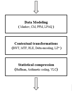
Modern compression tools and techniques are not based solely on the use of a data compression algorithm, actually the use of this is part of the final stage of an entire compression pipeline, but before reaching the last one, there is a stage called contextual transformations that are responsible for reorganizing the symbols of the dataset so they are more sensitive to statistical compression algorithms such as Huffman coding, two of the main algorithms that will be explained in this repository are the BWT and MTF.
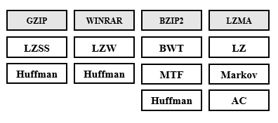
It should be noted that the Huffman algorithm is widely used in many known compression tools or codecs, the image below shows the compression pipelines of some of these tools and we can see that the huffman coding is very common in much of them
On the other hand, it is relevant to mention that Hadoop is one of the most famous tools to control and manage large amounts of data and is composed of the most robust codecs to compress its formats, most of these codecs are the tools mentioned below, for example in bzip2 the blocks can be decompressed independently, or they can be decompressed in parallel, making it a good tool to use in data-intensive solutions with distributed computing frameworks such as Hadoop, Apache Spark, and Hive. There is a considerable amount of studies on this, where the studies are based on improving the communication of these codecs with the main components of Hadoop. Internally these codecs use the contextual transformations mentioned in this document and others that were not mentioned, shows the codecs commonly used by Hadoop components, as mentioned before two of them use Huffman in their compression pipeline.
Before processing with the MTF algorithm, the sequence of symbols of the original dataset must go through the BWT algorithm first, this in order to improve the rate compression using the statistical encoding algorithm, below, an example of how its works using the following dataset: ABADBEAB
- The first input sequence is placed inside the first row of a matrix of size N * N, where N is the size of the sequence, the other rows have the same sequence, but each one cyclically rotated once to the left.
- The rows must be ordered lexicographically, the last highlighted column represents the BWT transformed string, in which repetitions of nearby symbols or clusters of symbols can be observed, the highlighted row represents the sequence of symbols from the original dataset.
The output of the BWT transformation algorithm for this example is expressed as follows: BWT = [I, S] where S represents the last column EBBAADAB and the value I = 1 represents the index of the row where the original sequence appears, both variables are needed to decode a sequence of symbols that was encoded with the BWT algorithm.
The reverse process can retrieve the original sequence of the dataset using the output variables of the previous process, I and S, the BWT decoding works as follows, it is iterated N times, where N is equal to the size of the sequence, in each iteration three actions occur that involve the following series of steps:
-
The sequence S is placed in a first column and the sequence S ordered lexicographically in a second column.
-
In the next iteration the first column is the concatenation of the first and second column of the previous step and the second column is the lexicographically ordered concatenation of the previous step and so on until iteration N.
-
The index I will tell us which is the correct sequence that represents the original dataset in iteration N.
The goal of this transformation technique is to improve the compression rate for a statistical compression algorithm, this method achieves better results when there are clusters of repeated symbols in the sequence being analyzed and normally this last feature is offered by the BWT, in chunks of the sequence of symbols of the original dataset there are always biases in the probabilities of the symbols, this means that locally there are repetitions of symbols and this is used by the MTF, its operation is described below using the output dataset of the algorithm BWT (EBBAADAB)
- We start with an ordered alphabet list, in this case the example is text-based, if we had images or other data where there is a larger alphabet it would not be a bad idea to use a byte-ordered list of all ASCII symbols.
- Each element in the ordered list must be easily identified by its index, this means that the first element in the list can be identified by index 0 and so on.
- At the moment of coding, if a symbol occurs the first time we must send the index corresponding to that symbol in the list, and the symbol is moved to the front of the list, the movements of the found index are stored for the output.
In this case, the output of the algorithm returns 4202412, a list of integers in small ranges, there is a probability that the union of the MTF-encoded chunks will have more repetitions and therefore less entropy, the compression with huffman benefits from this process, in In this example the entropy of the final sequence changed very little but above the BWT sequence, The decoder can recover the original sequence by reversing the process, given 4202412, it starts with an ordered list from A to Z and for each symbol that the decoder read, output the value at that index in the ordered list, then move that symbol to the front of the ordered list.
from scipy.stats import entropy
import seaborn as sns
import matplotlib.pyplot as plt
from collections import Counter
import pandas as pd
import numpy as npdef entropy_shannon(s, base=None):
v, c = np.unique(s, return_counts=True)
return entropy(c, base = base) def bw_transform(s):
n = len(s)
m = sorted([s[i:n]+s[0:i] for i in range(n)])
I = m.index(s)
L = [q[-1] for q in m]
return (I, L)
def bw_restore(I, L):
n = len(L)
X = sorted([(i, x) for i, x in enumerate(L)], key=itemgetter(1))
T = [None for i in range(n)]
for i, y in enumerate(X):
j, _ = y
T[j] = i
Tx = [I]
for i in range(1, n):
Tx.append(T[Tx[i-1]])
S = [L[i] for i in Tx]
S.reverse()
return ''.join(S) c_d = list(range(256))
def encodeMTF(plain_text):
dictionary = c_d.copy()
compressed_text = list()
rank = 0
for c in plain_text:
rank = dictionary.index(int(c))
compressed_text.append(rank)
dictionary.pop(rank)
dictionary.insert(0, int(c))
return compressed_text
def decodeMTF(compressed_data):
compressed_text = compressed_data
dictionary = c_d.copy()
plain_data = []
for rank in compressed_text:
plain_data.append(dictionary[rank])
e = dictionary.pop(rank)
dictionary.insert(0, e)
return plain_data def get_x_labels(s_v):
x_labels = []
for ix in range(len(s_v)):
if ix % 5 == 0:
x_labels.append(str(ix))
else:
x_labels.append('')
return x_labels
def plot(bts):
term_freq = Counter(bts)
n = len(term_freq)
N = sum(term_freq.values())
for term in term_freq:
term_freq[term] = term_freq[term] / N
df = pd.DataFrame.from_records(term_freq.most_common(n), columns = ['Byte', 'Frecuencia'])
fig = plt.figure(figsize = (18, 6))
ax = sns.barplot(x = 'Byte', y = 'Frecuencia', data = df.sort_values(by=['Byte']), color='#3498db')
plt.xticks(fontsize = 10, rotation = 60)
plt.title('Frecuencia de los bytes')
return plt def read_file(file_name):
with open(file_name, 'rb') as r:
original= bytearray(r.read())
return [x for x in original] originalbytes = read_file('book1-en.txt')
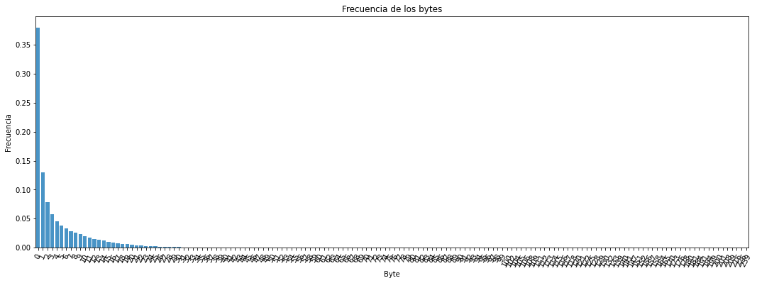
plt = plot(originalbytes)
plt.show()
print("Entropy:", entropy_shannon(originalbytes))Entropy: 3.1504021522329757
originalbytes = read_file('book1-en.txt')

slices_originalbytes = [originalbytes[i:i + 10000] for i in range(0, len(originalbytes), 10000)]

bw_ids = []
bytesbwt = []

for sc in slices_originalbytes:
    i, bw_slice = bw_transform(sc)
    bw_ids.append(i)
    bytesbwt.extend(bw_slice)

bytesMTF  = encodeMTF(bytesbwt)

plt = plot(bytesMTF)
plt.show()
print("Entropy:", entropy_shannon(bytesMTF))
Entropy: 2.449382298285078
RLE takes advantage of the succession of repeated symbols, also called clustered of symbols, a sequence of the same symbol is replaced by its number of repetitions and the symbol that is repeated, we call this type of replacement "RUN", see the following example:
In the example above we can clearly see that the algorithm in addition to offering a transformation offers compression, this algorithm also has its disadvantages when the repetitions of symbols are very short, it is advisable to read about the different implementations associated with this kind of contextual transformation.
from itertools import groupby

def rle_encoding(data):
    return [(len(list(k)), i) for i,k in groupby(data)]

def rle_decoding(ct):
    return ''.join(k * i for i,k in ct)

rle_encoding("RRRRRRRRRRunLLLLLLLLLLengthEEEEEEEEEEncode")
rle_decoding([(10, 'R'),(1, 'u'),(1, 'n'),(10, 'L'),(1, 'e'),(1, 'n'),(1, 'g'),(1, 't'),(1, 'h'),(10, 'E'),(1, 'n'),(1, 'c'),(1, 'o'),(1, 'd'),(1, 'e')])
check the below repository too:
@powturbo/Turbo-Run-Length-Encoding
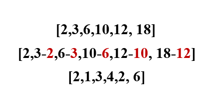
Sometimes there are local correlations between the data transmitted, for example in time-series, images or audio. It is absolutely necessary take advantage of the adjacency of each symbol, and sometimes could be very suitable, two adjacent values could describe one of them as the difference of the other value, subtract the current value from the previous one and store the difference in the same stream that is transmitted. This technique is called Delta Encoding and it is one of the most important algorithms regarding the compression and transmission of data means.
def delta_encode(data):
    l = 0
    for i in range(0, len(data)):
        c = data[i]
        data[i] = c - l
        l =  c

def delta_decode(data):
    l = 0
    for i in range(0, len(data)):
        delta = data[i]
        data[i] = delta + l
        l = data[i]

data = [3, 4, 5, 6]
delta_encode(data)
print(data)
delta_decode(data)
print(data)

[3, 1, 1, 1]
[3, 4, 5, 6]
XOR Delta encoding can deal with problems related to negative values, in addition to having the property of lowering the range of values, which in terms of entropy suits us.
def XOR_delta_encode(w):
    last = w[0]
    i = 1
    while(i< len(w)):
        c = w[i]
        w[i] ^= last
        last = c
        i += 1

def XOR_delta_decode(ct):
    last = ct[0]
    i = 1
    while(i< len(ct)):
        ct[i] ^= last
        last = ct[i]
        i += 1

data = [2,3,5,6,19, 20,31,15,7,8,4,10,20,5,10,12,5,8,93,120, 2, 5,5,3,20,5]

XOR_delta_encode(data)
print(data)
XOR_delta_decode(data)
print(data)

[2, 1, 6, 3, 21, 7, 11, 16, 8, 15, 12, 14, 30, 17, 15, 6, 9, 13, 85, 37, 122, 7, 0, 6, 23, 17]
[2, 3, 5, 6, 19, 20, 31, 15, 7, 8, 4, 10, 20, 5, 10, 12, 5, 8, 93, 120, 2, 5, 5, 3, 20, 5]
- When the differences between subsequent values is small Delta encoding could be suitable, in other cases negative values could be generated and this is bad.
- Xor delta encoding will not always lower the entropy of the symbol sequence, but it can help you to keep positive values in case the Delta encoding technique has generated negative values.
- If your data set does not has large repetitions of symbols, RLE won’t be suitable MTF could be a good option.
- MTF lowers the range of the values, thus offering a chain of symbols with less entropy, but the performance of this algorithm depends on a previous transformation that can create clusters of repeated symbols, the BWT can be a good option to generate these clusters.
- In cases where the nature of the dataset contains symbols with uniform distributions, for example images, the use of the BWT and MTF in the compression pipeline could help to achieve acceptable compression rates.
- BWT does not compress the data, you only will have a different permutation of the symbols that has consecutive repetitions and therefore a lower entropy.
Help me to improve this repository or just copy and paste my work
- Created by Ramses Alexander Coraspe Valdez
- Created Oct, 2020
This project is licensed under the terms of the MIT license.


