This repo contains my implementation for Logistic Regression, and examples on applying it to different datasets with
explanation for each example about data preprocessing step, and the learning algorithm behavior.
I made this repo to apply logistic regression on different data sets for better understanding of the algorithm and how it works, after completing the Neural Networks and Deep Learning course from deeplearning.ai taught by Andrew Ng. on coursera, Certificate.
Logistic Regression is a supervised learning technique that is used for binary classification problems, where the dataset
conatins one or more independant varibales that determine a binary outcome (0 or 1).
In a logistic regression classifier, you may want to input a feature vector X which describes the features for a single row of data,
and you want to predict a binary output value which is either 0 or 1.
More formally, given an input vector X, you want to predict y_hat which is an output vector describing the probability that y = 1 given
feature vector X, y_hat = p(y = 1 / X).
You have an input vector X, where the features are gender, age and salary for a specific person, and you want to predict whether or not this person will purchase a specific product or not.
The training dataset will contain rows of data, where each row represents a tuple of (X, y), where:
- X is a n_x dimentional vector (n_x is the number of independant varibales discribing the row of data).
- y is a binary value, whether 0 or 1, describing whether or not the user has purchased the product.
In order to train the Logistic Regression Classifier, we'll divide our dataset into training and test sets, having m training examples.
We'll then stack every training example X(i) as column vectors in a large input matrix of shape (n_x, m), and also stack the output
values y as columns in a large output matrix of shape (1, m).
We'll have also to initalize a weights vector and a bias which are learnable, and both will allow the classifier to learn and extract
features and paterns from the input data.
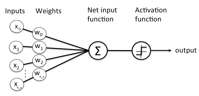
Then all what is left to do is to feed this data into our Logistic Regression Classifier, the image below describes how to the data is fed
to the classifier.
The Forward Propagation step:
Taking the dot product of a given feature vector and the vector of weights in addition to the bias term, will result in a single value output that describes the contribution of the initialized weights in the result of the classifier.
But this output value does not represent any expected value, neither 0 or 1, that's why we have to pass this value into another function that will map this value to another value between 0 and 1.
Here comes the power of the activation function.
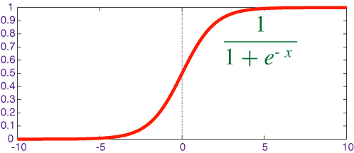
There is a function that we will use that will easily map any real value to a value between 0 and 1, which is the Sigmoid Activation Function.
Then we can put a threshold value as 0.5, if the sigmoid output is bigger than 0.5, then the prediction result is 1, else the prediction is 0. ```python def sigmoid(x): return 1 / (1 + np.exp(-x)) y_hat = sigmoid(np.dot(W.T, X) + b) y_hat[y_hat > 0.5] = 1 y_hat[y_hat <= 0.5] = 0 ```
We use the gradient descent algorithm to get the amount of contribution of each of the weights in the total error. This amount of contribution is represented in the dot product of X and the transpose of the subtraction of the activation result and the actual result in the output matrix, then we divide over m to get the average over all m training examples.
Also we compute the amount of contribution of the bias in the error by doing the summation of the differences between the activation result and the actual result y vector, also averaged by all m training examples.
dw = (1 / m) * np.dot(X, (y_hat - y).T)
db = (1 / m) * np.sum((y_hat - y))
The weight and bias update is a simple operation of subtracting the gradients from the vector of weights and bias to get better weights that can model input vectors to outputs with better accuracy.
To compute the cost of the minimization function for the algorithm, which is the log likelihood function, we compute the loss for every training example, which can be computed as
loss = (np.sum(y * np.log(y_hat)) + (1 - y) * np.log(1 - y_hat)))where y is the actual output of the input vector, and y_hat is the predicted output result from the forward propagation step. Then we can compute the cost by summing all the losses over all m training examples, and then averaging them by m.
cost = (-1 / m) * (np.sum(y * np.log(y_hat) + (1 - y) * np.log(1 - y_hat)))To create a new object of the classifier, you have to specify:
- The input and output matrices.
- The learning rate, which will control how big will the gradient descent step will be.
- The number of epochs the classifier will train.
- Boolean value which will indicate if the class will plot a graph for the learning process or not.
logistic_regression_object = LogisticRegression(X_train, Y_train, 0.5, 2500, True) Then call the function optimize to begin the learning process.
logistic_regression_object.optimize()You can get the confusion matrix using get_confusion_matrix function.
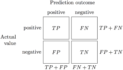
confusion_matrix = logistic_regression_object.get_confusion_matrix()The confusion matrix is the matrix that contains the result of the performance of your classifier.
This is how a confusion matrix is organized:
You can get the accuracy by calculating the following ```python accuracy = (confusion_matrix[0, 0] + confusion_matrix[1, 1]) / np.sum(confusion_matrix) ``` You can also get the weights vector and bias using **get_weights** and **get_bias** functions.


