Image of Natural Scenes Classification
(Intel Image classification Challenge)
build from scratch and use pre-trained models

In neural networks, Convolutional neural network (ConvNets or CNNs) is one of the main categories to do images recognition, images classifications. Objects detections, recognition faces etc., are some of the areas where CNNs are widely used.
The name “convolutional neural network” indicates that the network employs a mathematical operation called convolution. Convolutional networks are a specialized type of neural networks that use convolution in place of general matrix multiplication in at least one of their layers.
CNN image classifications takes an input image, process it and classify it under certain categories. Computers sees an input image as array of pixels and it depends on the image resolution. Based on the image resolution, it will see h x w x d( h = Height, w = Width, d = Dimension ). Eg., An image of 6 x 6 x 3 array of matrix of RGB (3 refers to RGB values) and an image of 4 x 4 x 1 array of matrix of grayscale image.
CNNs are regularized versions of multilayer perceptrons. Multilayer perceptrons usually mean fully connected networks, that is, each neuron in one layer is connected to all neurons in the next layer. The "fully-connectedness" of these networks makes them prone to overfitting data. Typical ways of regularization include adding some form of magnitude measurement of weights to the loss function.

When programming a CNN, the input is a tensor with shape (number of images) x (image height) x (image width) x (image depth). Then after passing through a convolutional layer, the image becomes abstracted to a feature map, with shape (number of images) x (feature map height) x (feature map width) x (feature map channels). A convolutional layer within a neural network should have the following attributes:
- Convolutional kernels defined by a width and height (hyper-parameters)
- The number of input channels and output channels (hyper-parameter)
- The depth of the Convolution filter (the input channels) must be equal to the number channels (depth) of the input feature map
Convolutional networks may include local or global pooling layers to streamline the underlying computation. Pooling layers reduce the dimensions of the data by combining the outputs of neuron clusters at one layer into a single neuron in the next layer. Local pooling combines small clusters, typically 2 x 2. Global pooling acts on all the neurons of the convolutional layer.In addition, pooling may compute a max or an average:
- Max pooling uses the maximum value from each of a cluster of neurons at the prior layer
- Average pooling uses the average value from each of a cluster of neurons at the prior layer
Fully connected layers connect every neuron in one layer to every neuron in another layer. It is in principle the same as the traditional multi-layer perceptron neural network (MLP). The flattened matrix goes through a fully connected layer to classify the images.
The input area of a neuron is called its receptive field. So, in a fully connected layer, the receptive field is the entire previous layer. In a convolutional layer, the receptive area is smaller than the entire previous layer. The subarea of the original input image in the receptive field is increasingly growing as getting deeper in the network architecture.
Each neuron in a neural network computes an output value by applying a specific function to the input values coming from the receptive field in the previous layer. The function that is applied to the input values is determined by a vector of weights and a bias (typically real numbers). Learning, in a neural network, progresses by making iterative adjustments to these biases and weights. The vector of weights and the bias are called filters and represent particular features of the input (e.g., a particular shape). A distinguishing feature of CNNs is that many neurons can share the same filter. This reduces memory footprint because a single bias and a single vector of weights are used across all receptive fields sharing that filter, as opposed to each receptive field having its own bias and vector weighting.
The intuition behind transfer learning for image classification is that if a model is trained on a large and general enough dataset, this model will effectively serve as a generic model of the visual world. We can then take advantage of these learned feature maps without having to start from scratch by training a large model on a large dataset.
Transfer learning is an optimization, a shortcut to saving time or getting better performance. In general, it is not obvious that there will be a benefit to using transfer learning in the domain until after the model has been developed and evaluated. Lisa Torrey and Jude Shavlik in their chapter on transfer learning describe three possible benefits to look for when using transfer learning:
- Higher start -- The initial skill (before refining the model) on the source model is higher than it otherwise would be
- Higher slope -- The rate of improvement of skill during training of the source model is steeper than it otherwise would be
- Higher asymptote -- The converged skill of the trained model is better than it otherwise would be
ResNet(Residual Networks)-50 is is a variant of ResNet model which has 48 Convolution layers along with 1 MaxPool and 1 Average Pool layer. We can load a pretrained version of the network trained on more than a million images from the ImageNet database. A ResNet50 model was pretrained on a million images from the ImageNet database and can classify images into 1000 object categories. As a result, the network has learned rich feature representations for a wide range of images. The network has an image input size of 224-by-224. The fundamental breakthrough with ResNet was it allowed us to train extremely deep neural networks with 150+layers successfully. Prior to ResNet training very deep neural networks was difficult due to the problem of vanishing gradients.
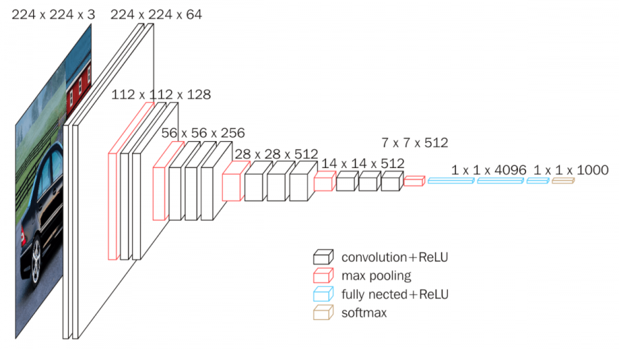
VGG(Visual Geometric Group)16 is a convolutional neural network model proposed by K. Simonyan and A. Zisserman from the University of Oxford in the paper “Very Deep Convolutional Networks for Large-Scale Image Recognition”. The model achieves 92.7% top-5 test accuracy in ImageNet, which is a dataset of over 14 million images belonging to 1000 classes. It was one of the famous model submitted to ILSVRC-2014. The 16 in VGG16 refers to it has 16 layers that have weights. These 16 layers contain the trainable parameters and there are other layers also like the Max pool layer but those do not contain any trainable parameters. This network is a pretty large network and it has about 138 million (approx) parameters.
Inception-v3 is a convolutional neural network architecture from the Inception family that makes several improvements including using Label Smoothing, Factorized 7 x 7 convolutions, and the use of an auxiliary classifer to propagate label information lower down the network (along with the use of batch normalization for layers in the sidehead). By rethinking the inception architecture, computational efficiency and fewer parameters are realized. With fewer parameters, 42-layer deep learning network, with similar complexity as VGGNet, can be achieved. With 42 layers, lower error rate is obtained and make it become the 1st Runner Up for image classification in ILSVRC (ImageNet Large Scale Visual Recognition Competition) 2015. Inception-V3 was trained using a dataset of 1,000 classes from the original ImageNet dataset which was trained with over 1 million training images, the Tensorflow version has 1,001 classes which is due to an additional "background" class not used in the original ImageNet.