This is a notebook showing how to use the code of the proposed method for Multi-Centrality Index, which was employed for the analysis of keywords in [1]. The code is in Python3, and some toolboxes are necessary to run the commands.
The following very common packages are necessary for running the code:
- numpy
- pandas
- networkx
- sklearn
import numpy as np
import pandas as pd
import networkx as nx
from sklearn.decomposition import PCA
from sklearn.preprocessing import StandardScaler, MinMaxScaler
Then, you can run the example from a preloaded matrix of features (centralities) of a previous constructed graph-of-words (network) with the co-occurrence approach.
Each word of the graph is sorted by the corresponding Multi-centrality Index (MCI) value. In this example, the MCI is the combination of these centrality measures: ['Degree','Pagerank','Eigenvector','StructuralHoles']
Top words are considered the keywords of the text.
You run the code as follow:
python MultiCentralityIndex.py Word MCI
0 MAMET 1.501088
1 PLAY 1.484412
2 DIRECTOR 0.968968
3 ANARCHIST 0.887786
4 THEATER 0.712872
5 PULITZER 0.647991
6 LONDON 0.635058
7 GOOLD 0.619282
8 YEAR 0.605723
9 GLENGARRY 0.572361
10 DEBUT 0.530749
11 DAVID 0.311259
12 YORK 0.225655
13 PRIZEWINNER 0.215347
14 PRIZE 0.208866
...
import MultiCentralityIndex as mc
mc.test()
Besides, you can import and use the code as your necessity. For example, lets calculate the MCI for the Coauthorships in network science
| A figure depicting the largest component of this network Extracted from Prof. Newman Web site | 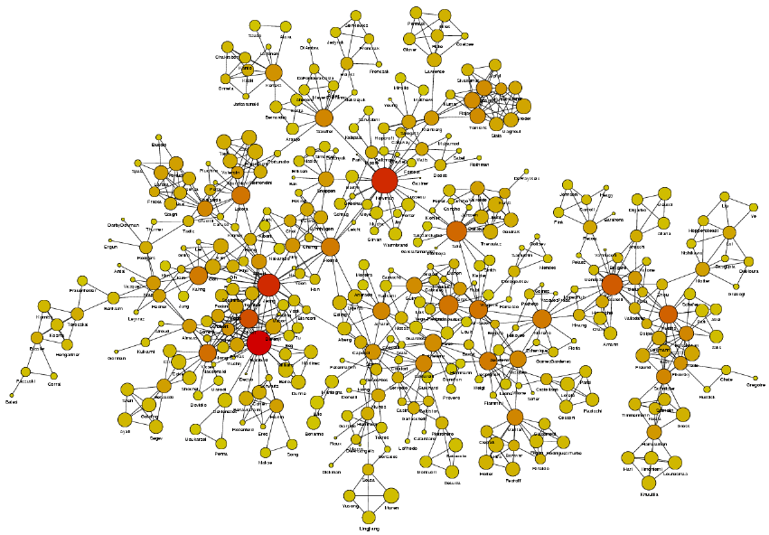 |
import MultiCentralityIndex as MCI
import networkx as nx

# Creating the MCI object
mc = MCI.MCI()

#loading the netscience graph
G = nx.read_gml('netscience.gml',label='label')
node_size=[float(G.degree(v)) for v in G]

#Showing the graph of the full network
nx.draw_networkx(G, arrows=True, node_size=20, node_color=node_size,edge_color='grey',alpha=.5,with_labels=False)
Now, let's define the set of centrality measures to be calculated as
setCentralities = ['Degree','Pagerank','Eigenvector','StructuralHoles','Closeness', 'Betweenness']In this example we are calculating the MCI for a single graph (network). For this, we just call the getMCI_PCA method.
mc.getMCI_PCA(G,setCetralities=setCentralities)[:10]| Word | MCI | |
|---|---|---|
| 0 | NEWMAN, M | 1.550027 |
| 1 | BARABASI, A | 1.330304 |
| 2 | JEONG, H | 1.221634 |
| 3 | PASTORSATORRAS, R | 1.043823 |
| 4 | SOLE, R | 1.040874 |
| 5 | BOCCALETTI, S | 0.978564 |
| 6 | MORENO, Y | 0.903129 |
| 7 | HOLME, P | 0.871221 |
| 8 | CALDARELLI, G | 0.808137 |
| 9 | VESPIGNANI, A | 0.807601 |
Note: In the case of ref[1], we calculated the matrix of features from a collection or set of graphs-of-words of a repository and, then, we computed the first Principal Component (getPC1 method) from this matrix of features of the entire repository
Behind the scene, the getMCI_PCA is calling the getPC1FromGraph method, which obtains the matrix of centrality measures of the graph (mtxDoc) and calls the getPC1 function for computing the first Principal Component (PC1) of the graph.
For illustration purpose, this is the matrix of features of the graph:
mtxDoc = mc.getMatrixFeaturesGraph(G,setCentralities)
display(mtxDoc)| Word | Degree | Pagerank | Eigenvector | StructuralHoles | Closeness | Betweenness | |
|---|---|---|---|---|---|---|---|
| 0 | ABRAMSON, G | 0.0588 | 0.1398 | 1.418e-15 | 0.8871 | 0.0231 | 0.000000 |
| 1 | KUPERMAN, M | 0.0882 | 0.2209 | 1.410e-15 | 0.5085 | 0.0309 | 0.000071 |
| 2 | ACEBRON, J | 0.1176 | 0.1425 | 1.394e-15 | 0.6565 | 0.0412 | 0.000000 |
| 3 | BONILLA, L | 0.1176 | 0.1425 | 1.396e-15 | 0.6565 | 0.0412 | 0.000000 |
| 4 | PEREZVICENTE, C | 0.1176 | 0.1425 | 1.419e-15 | 0.6565 | 0.0412 | 0.000000 |
| ... | ... | ... | ... | ... | ... | ... | ... |
| 1584 | MONDRAGON, R | 0.0294 | 0.1425 | 1.403e-15 | 0.8805 | 0.0103 | 0.000000 |
| 1585 | ZHU, H | 0.0588 | 0.2196 | 1.405e-15 | 0.4027 | 0.0206 | 0.000035 |
| 1586 | HUANG, Z | 0.0294 | 0.1040 | 1.407e-15 | 0.8805 | 0.0137 | 0.000000 |
| 1587 | ZHU, J | 0.0294 | 0.1040 | 1.409e-15 | 0.8805 | 0.0137 | 0.000000 |
| 1588 | ZIMMERMANN, M | 0.0588 | 0.0731 | 1.422e-15 | 0.5524 | 0.1381 | 0.000000 |
1589 rows × 7 columns
And this is the first Principal Component (PC1) of the graph according to all columns (centralities) in the matrix of features
PC1 = mc.getPC1(mtxDoc)
print(PC1)
Degree Pagerank Eigenvector StructuralHoles Closeness Betweenness
0 0.535797 0.434088 0.202644 -0.494563 0.329897 0.360556
Or, you can filter selecting specific centralities
PC1 = mc.getPC1(mtxDoc,setCentralities=['Degree', 'Pagerank', 'StructuralHoles'])
print(PC1)
Degree Pagerank StructuralHoles
0 0.621633 0.532563 -0.574412
Now, we can calculate the MCI of the graph considering the previous PC1 and calling the function
N = 10
centralNodes = mc.getMCI_PCA(G, PC1, N=N)
where N means the top N nodes. If N = -1 it returns all the nodes.
N = 10
MCI = mc.getMCI_PCA(G, PC1, N=N)
display(MCI)| Word | MCI | |
|---|---|---|
| 0 | BARABASI, A | 1.091113 |
| 1 | NEWMAN, M | 1.026212 |
| 2 | JEONG, H | 0.829966 |
| 3 | YOUNG, M | 0.623524 |
| 4 | OLTVAI, Z | 0.603774 |
| 5 | BOCCALETTI, S | 0.601977 |
| 6 | SOLE, R | 0.567841 |
| 7 | KURTHS, J | 0.519397 |
| 8 | ALON, U | 0.510426 |
| 9 | PASTORSATORRAS, R | 0.492352 |
Clearly, the ranking changes depending on the selected centrality measures. This is why our proposal in Ref[1] of finding the best subset of centralities according to your supervised problem. For instance, applying some Feature Selection methods, correlation analysis, etc.
In unsupervised problems, a good approach could be to select the group of centrality measures less correlated.
TextMiner is a module that employs the MCI for extracting keywords and keyphrase from a single or collection of texts.
For using, you will need to have nltk and itertools packages installed:
os, re, string, nltk, en_core_web_sm, itertools, collectionsFollowing, an example of use:
import TextMiner as tm
import en_core_web_sm

Miner = tm.TextMiner(punctuations=None,min_length_sent=7, nlp=en_core_web_sm.load())
Miner.candi_pos = ['NOUN', 'PROPN', 'ADJ']

# number of returned keywords and keyphrases
N = 10

# Loading three examples of stories written by Edgar Allan Poe
# content[0] is the "The Black Cat" story
from data.content import content

#Case 1. Considering a single text
keywords = Miner.get_keywords_MCI_from_text(content[0],numberKeyWords=N)


print('CASE 1: \n\t Keywords\n')
print(keywords)
print('\n \t Keysentences \n')

for sentence in Miner.get_ranked_phrases()[:N]:
    print('----------\n',sentence)

print('\n\t\t================ || =================\n')

#Case 2. Considering a collection of texts
mtxDoc = Miner.get_mtxDoc_from_collection(content,
                                          setCentralities=['Degree',
                                                        'Pagerank',
                                                        'StructuralHoles'])

keywords = Miner.get_keywords_MCI_from_text(content[0],mtxDoc=mtxDoc,
                                            numberKeyWords=N)
print('CASE 2: \n \t Keywords\n')
print(keywords)
print('\n \t Keysentences \n')

for sentence in Miner.get_ranked_phrases()[:N]:
    print('----------\n',sentence)
print('-------')
CASE 1:
Keywords
Word MCI
0 mere 1.933236
1 half 1.337548
2 horror 1.005507
3 cat 0.979326
4 other 0.973901
5 beast 0.971519
6 such 0.847697
7 reason 0.845035
8 terrible 0.844638
9 humanity 0.833198
Keysentences
----------
half of horror and half of triumph
----------
which goes directly to the heart of him who has had frequent occasion to test the paltry friendship and gossamer fidelity of mere man
----------
i indeed wretched beyond the wretchedness of mere humanity
----------
mournful and terrible engine of horror and of crime
----------
and many persons seemed to be examining a particular portion of it with very minute and eager attention
----------
i experienced a sentiment half of horror
----------
my next step was to look for the beast which had been the cause of so much wretchedness
----------
and which constituted the sole visible difference between the strange beast and the one i had destroyed
----------
this dread was not exactly a dread of physical evil
----------
that the terror and horror with which the animal inspired me
================ || =================
CASE 2:
Keywords
Word MCI
0 mere 1.253141
1 half 0.947709
2 beast 0.819257
3 cat 0.787077
4 other 0.687237
5 many 0.650715
6 more 0.650715
7 white 0.638784
8 wall 0.626681
9 sense 0.613148
Keysentences
----------
half of horror and half of triumph
----------
which goes directly to the heart of him who has had frequent occasion to test the paltry friendship and gossamer fidelity of mere man
----------
i indeed wretched beyond the wretchedness of mere humanity
----------
this dread was not exactly a dread of physical evil
----------
i experienced a sentiment half of horror
----------
there came back into my spirit a half
----------
that the terror and horror with which the animal inspired me
----------
and many persons seemed to be examining a particular portion of it with very minute and eager attention
----------
for no other reason than because he knows he should not
----------
and which for a long time my reason struggled to reject as fanciful
-------
In CASE 1, the base of knowledge is extracted from the same text. The get_keywords_MCI_from_text implicitly construct the matrix of word features from content[0], which is used to extract the MCI keywords.
In CASE 2, the matrix of word features is constructed from the entire collection of text, by using the get_mtxDoc_from_collection method. Then, the matrix of word features (mtxDoc) is passed as parameter for finding the MCI keywords in content[0].
You can use this code as it is for academic purpose. If you found it useful for your research, we appreciate your reference to our work A multi-centrality index for graph-based keyword extraction:
[1] Didier A. Vega-Oliveros, Pedro Spoljaric Gomes, Evangelos E. Milios, Lilian Berton. Information Processing & Management, V. 56, I. 6, November 2019, 102063. https://doi.org/10.1016/j.ipm.2019.102063