machine_translator

Introduction

What is the meaning behind a text? How do we humans interpret it? It definitely feels like a straightforward thing for us to infer meaning out of text, but is it really that straightforward? What was the necessary process we had to go through to internalize the implicit rules that led us to the point that we could read? That is what nature's analog machine, consisted of a sizeable set of interconnected biological neurons (~100 billion nodes, ~100 trillion connections), is capable of. That is what the human brain does, and given the rate of technological advancement and the exponential rate of data availability, it is only a matter of time before humans will completely unearth its hidden powers.

A sentence can be interpreted in multiple ways and expressed in even more ways. Because of that, the boundary between a right and a wrong translation is fuzzy. As a result, we expect that the very nature of the translation problem to intrinsically employ an unavoidable error. The error of lexical ambiguity. This kind of error is comparable to the inevitable noise that measurement devices capture. Thankfully neural networks and their training processes are able to bypass such errors under normal circumstances.

Recent Developments

State of the art sequence-to-sequence models [1,2,3] have recently taken the spotlight in both the industrial and academic sectors. The increasing attractiveness of these technologies has led to a shift in business models, emergence of market disruptions, and the rise of new rivalries [4]. The central trigger of this chain of events seems to be OpenAI's revolutionary chatbot called ChatGPT [1], starting around Q4 of 2022, when it was first released to the public as a free product.

The context of word definitions, their connotation and grammatical rules are some of the major features that these sophisticated models have been trained to capture almost flawlessly. This is more than enough evidence that the encoder-decoder pipeline (see Figure 1), the backbone of all these popular transformer models, offers a promising solution to extremely complex text processing tasks. A backbone that holds the potential to refine a highly generalizable distribution function, from massive amounts of sequence-to-sequence data. Text translations, text-to-voice and chat conversations are some of many relevant applications. Our focus here will be the former due to its manageable requirement in hardware quality and data size.

Figure 1. Source [1]. The encoder-decoder pipeline.

Overview of machine_translator

The current project is a highly configurable tool, suitable for training machine translation models that utilize the encoder-decoder neural network pipeline. It is a PyTorch based software developed to run on a system equipped with a python interpreter (or a Jupyter Kernel) and a GCC compiler. In order to achieve making it more configurable, an attempt was made to avoid relying on high abstraction functions (e.g. the forward method of a layer's sub-module), hence most of the basic functions were implemented from scratch. The primary reason that PyTorch was utilized was to invoke the automatic differentiation mechanism that its graph system provides.

It goes without saying that althought the current project's approach takes advantage of modern methodologies, it achieves trivial results compared to masterpieces like Google Translate [5] or DeepL Translator [6]. machine_translator's development was heavily relied on Dive into Deep Learning [7]. A model has been trained in order to demonstrate the software's capabilities and limitations, as well as to gain some insights about sequence-to-sequence processing in general.

English to Greek Translation

The task at hand is the translation of sentences between the english and greek languages. To achieve this, we have used a dataset we refer to as ell.

Raw ell Dataset

The ell dataset [8] is consisted of sentence translations between the english and greek languages. Its file is encoded in UTF-8 with path ./datasets/ell.txt. The following block shows a small chunk of it, consisting of 3 translation pairs.

...
She has five older brothers.	Έχει πέντε μεγαλύτερους αδερφούς.	CC-BY 2.0 (France) Attribution: tatoeba.org #308757 (CK) & #1401904 (enteka)
She intended to go shopping.	Σκόπευε να πάει για ψώνια.	CC-BY 2.0 (France) Attribution: tatoeba.org #887226 (CK) & #5605459 (Zeus)
She left her ticket at home.	Άφησε το εισιτήριο στο σπίτι.	CC-BY 2.0 (France) Attribution: tatoeba.org #315436 (CK) & #7796665 (janMiso)
...

The file that is primarily responsible for the parsing of the dataset as well as its preprocessing, is ./src/dataset.py.

Initial Corpus Preprocessing

Obviously, the part that begins with CC-BY 2.0 was dropped from the raw text. The characters ,.!?; are all considered as tokens. No grammatical structure is explicitly considered here, hence words like walk and walking, although they share the same base word, will be treated as two distinct word entities.

Main Corpus Preprocessing

We shall refer to the english sentences as the source sequences, and the greek sentences as the target sequences. Hence in the above example, the following are the source sequences

She has five older brothers .
She intended to go shopping .
She left her ticket at home .

with corresponding target sequences

Έχει πέντε μεγαλύτερους αδερφούς .
Σκόπευε να πάει για ψώνια .
Άφησε το εισιτήριο στο σπίτι .

Additionally, a token (i.e. the smallest unit inside a sequence associable with a context) will be treated as equivalent to a word.

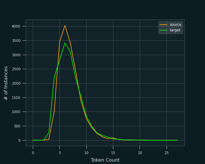
The preceding definitions now allow us to inspect the data from a clear viewpoint. In total, there are 17499 translations with varying sequence sizes, where the majority of them ranges from 4 to 11 tokens per sentence (see Figure 2).

To simplify the processing of data, all the preprocessed sequences in each language share the same length. The two distributions of Figure 2 seem to be almost identical, hence it makes sense to set the same length for both languages. That max_steps_seq length is set to be 9. All sequences that had more than 9 tokens were cropped to match this length, while all sequences that had less than 9 tokens, were filled with a repeating padding token <pad> until the size was 9. Additionally, for all sequences, before their paddings (if they have any), end with the special end of sequence token <eos>.

Figure 2. Displays how many sequences share a common number of tokens in both the source language (english) and the target language (greek).

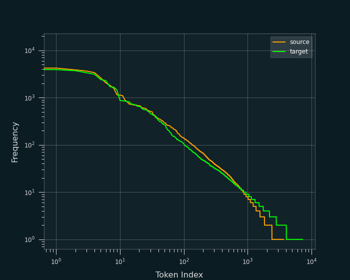
Inferring the context of a low-frequency token can be challenging because there are not enough sequences to provide information about its meaning. These rare instances of a token are outliers that can mislead the training process, resulting in solution-models that are more susceptible to issues such as overfitting and reduced overall performance. An additional problem is that these low frequency tokens add to the model's complexity. Specifically the vocabularies' increase, forces an unnecessary enlargement of the sequence-to-sequence model, hence increasing the time required for its training to converge in satisfying solutions, and given that it's more prone to overfitting, that solution is not worth the extra wait. In ell, the frequency of token appearances is shown in Figure 3.

As a result, it was decided that all tokens with frequency less than or equal to 1 were redundant and hence were replaced by the special token <unk>. Hence the sequences

Έχει πέντε μεγαλύτερους αδερφούς .
Ο Τομ και η Μαίρη επιτέλους αποφάσισαν να παντρευτούν .

now may look like

Έχει πέντε μεγαλύτερους αδερφούς . <eos> <pad> <pad> <pad>
Ο Τομ και η Μαίρη <unk> αποφάσισαν να <eos>

Do not forget that the punctuation mark . is a separate token in each of these vocabularies.

Figure 3. These plots display the relations between token indices and the number of their instance-appearance inside the dataset, in logarithmic scale. Each number on the horizontal axis represents a token's index sorted in decreasing order with respect to their frequency of appearance inside the dataset.

The resulting integer-index vocabularies were built with respect to the token frequency sorted in a decreasing order. Hence words like the will have a far lower index than the word ticket. One hot encoding (OHE) was incorporated minibatch-wise during the training, instead of prior to the training, due to the excessive memory requirement.

Some of these preprocessing routines used on the dataset are computationally demanding and conventional python routines are substantially slowing down the initialization of trainings. That is where C and ctypes come in handy. The more demanding preprocessing transformations were handled by ./src/preprocessing_tools.c, offering processing speedups up to $\times287$. These transformations are

• arstr2num: Conversion of all the dataset's strings into vocabulary indices.
• pad_or_trim: Sequence padding and sequence trimming.

The resulting vocabularies have sizes

• Source vocabulary size (src_vocab_size): 2404 .
• Target vocabulary size (tgt_vocab_size): 4039 .

Also the dataset is shuffled and split into a training and a validation set with ratio $90%$ versus $10%$.

Finally, as soon as the data preprocessing finishes, a torch.utils.data.TensorDataset object holding the entire preprocessed dataset is saved in ./datasets/pp_ell.pt.

Architectures and Training Process

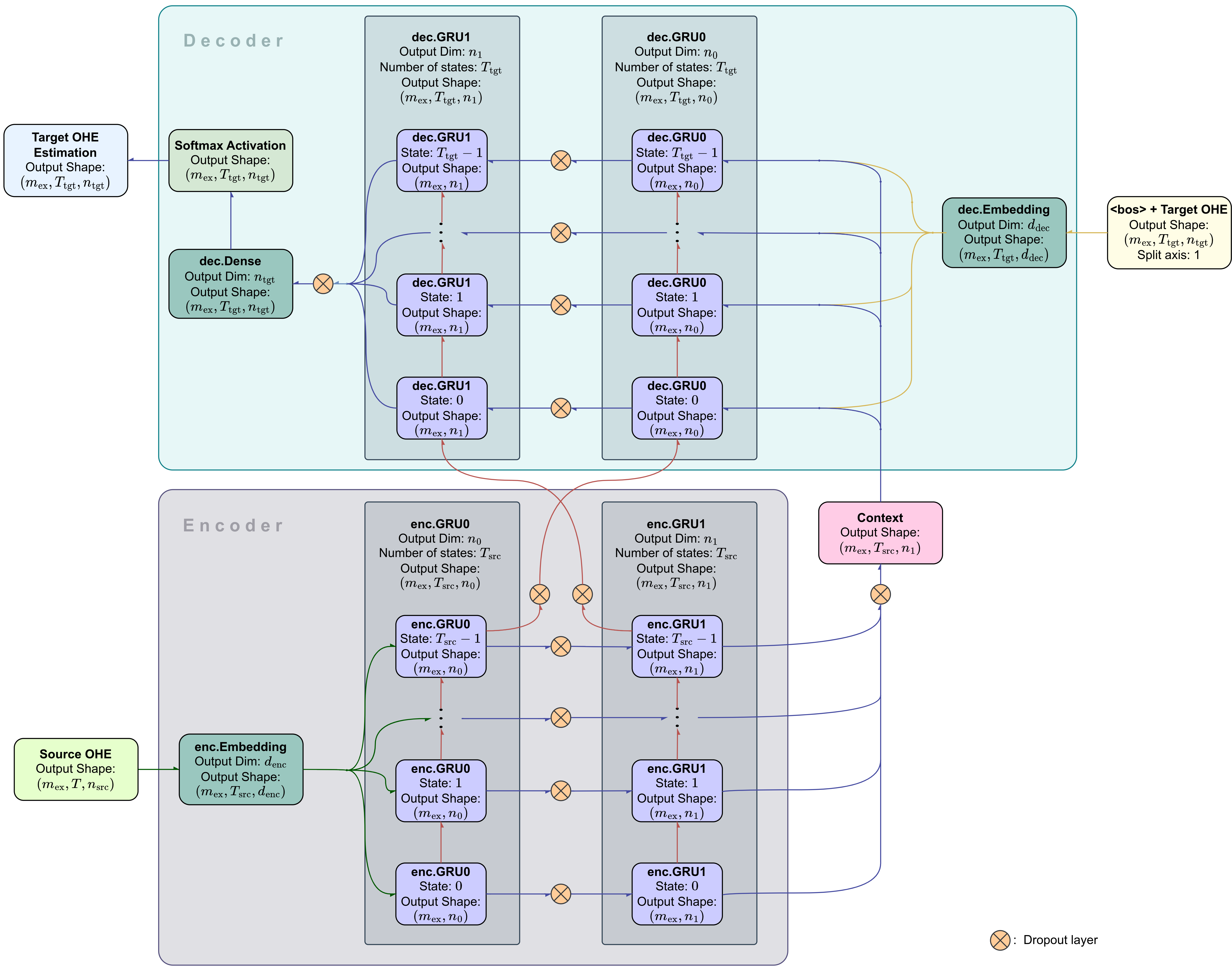
After an extensive effort of hyperparameter tuning, the following design was selected to carry out the training. The trainable pipeline is a teacher forcing encoder-decoder RNN specified in Figure 4. This particular pipeline will be named as s2s_ell_train. Each of the decoder's initial states were set to be the special beginning-of-sequence token <bos>.

The RNN's architecture is consisted of GRUs and dense layers, where each was set to output 600 neurons, except from the output layer with output size equal to 4039 (size of the target vocabulary). The dense layers were used as embedding layers in both the encoder and decoder, the target language's sequence reconstruction layer towards the end of the pipeline, and the decoder's output layer right after that reconstruction layer. On the other hand, GRUs have been proven beneficial as hidden layers, as they effectively infer the input sequence's context while incorporating temporal information. The output layer (i.e. the decoder's output layer) uses the Softmax activation function to produce the target vocabularies distribution.

Both the encoder and decoder consist of 2 stacked GRU layers. All of the encoder GRUs' initial states are set to zero tensors, while the decoder GRUs' initial states are set as the corresponding final states of the encoder's GRU layers. Hence, the initial state of the decoder's first GRU layer is assigned to be the final state of the encoder's first GRU layer, while the initial state of the decoder's second GRU layer is assigned to be the final state of the encoder's second GRU layer. Another design choice is that the context tensor is assigned as the output tensor produced by the final layer of the encoder. During decoding, for a given state, the context tensor is concatenated with the previous state's output along the token-wise feature axis.

From the trainable parameters of these layers, each bias $\mathcal{B}$ was initialized to a zero tensor and each weight $\mathcal{W}$ was sampled from a uniform Xavier distribution. Specifically $$\mathcal{W} \sim U(-b,b)$$ where $$b := \sqrt{3} \cdot \sqrt{\frac{2}{k_{\text{in}}+k_{\text{out}}}}$$ with $k_{\text{in}}$ and $k_{\text{out}}$ being the current layer's number of input and output neurons per state.

Figure 4. The teacher forcing s2s_ell pipeline. All dropout layers were shut down during the training.

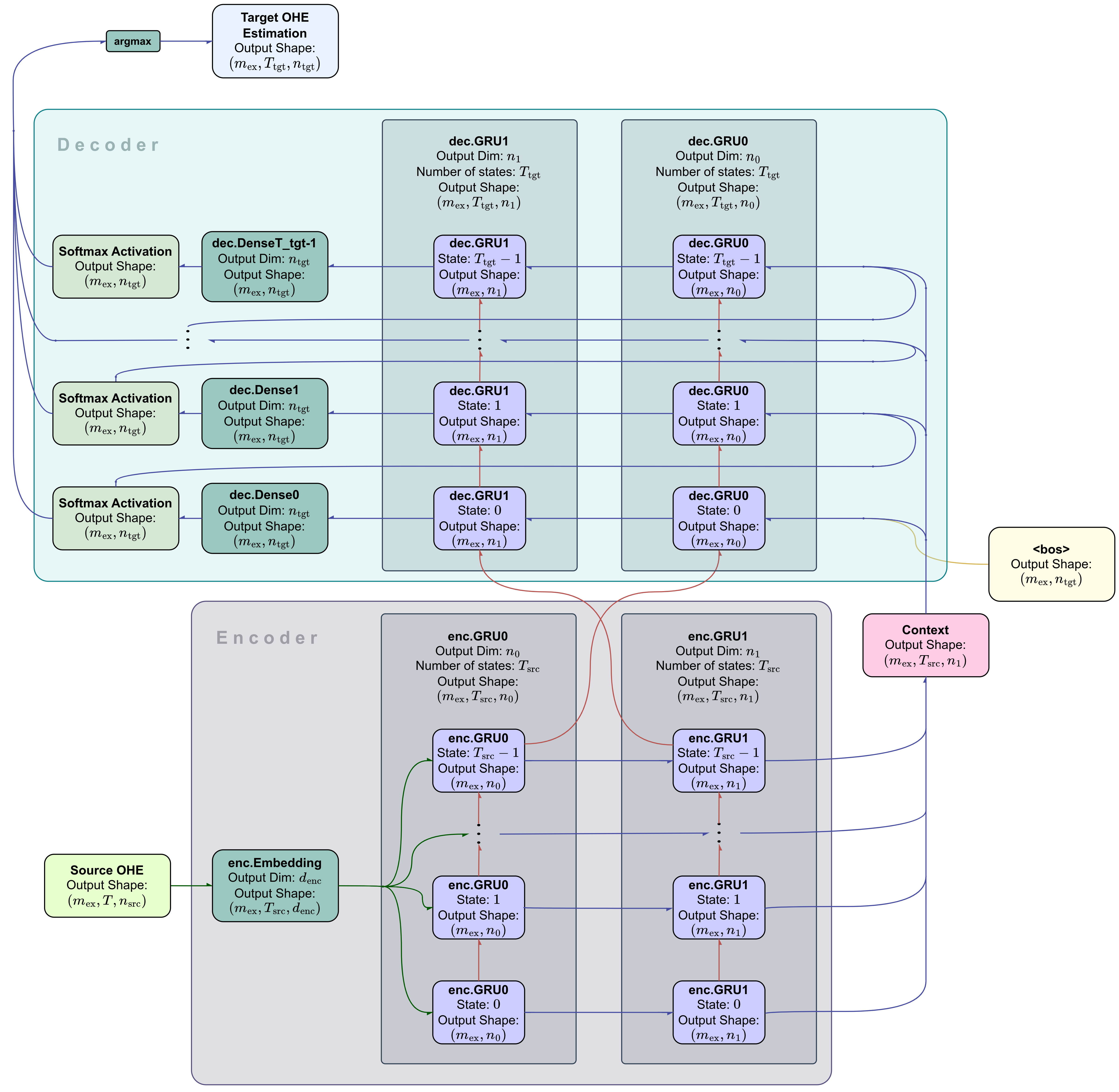
During testing, the pipeline depicted in Figure 4 obviously cannot predict sequences with unknown target outputs because the decoder has no available predefined decoder-inputs (or targets). Figure 5 shows the autoregressive pipeline of s2s_ell used for predictions, which is the version of s2s_ell intended to be trained during the training process. We'll refer to this pipeline as s2s_ell_pred. For each $t \in \{ 0, \dots, 9-1 \}$ of the decoder's state, the decoder's input is assigned to be the output distribution $\hat{f}_{t-1}$ of its corresponding previous state $t-1$. This resembles the deterministic greedy search approach where each state $t$ accepts a token $\text{argmax}_{ j }(\hat{f}_{t-1})$, where $j \in \{ 0, \dots, 4039-1 \}$.

Figure 5. s2s_ell predicts using this pipeline, allowing for the final model's predictions. Its usage extends on the model's evaluation. It's worth noting that the parameters of dec.Dense (from Figure 4), dec.Dense1, dec.Dense2, ..., dec.DenseT_tgt-1 are all the same.

For s2s_ell's trainable parameter updates, Adam is the responsible optimization algorithm that was selected for this training. The initial learning rate of Adam was set to 0.005 and for each training step, the minibatch size was set to 2¹⁰. Categorical cross entropy was selected to be the trainer's loss function, as it works well with the output layer's softmax activation. Furthermore, to prevent potential gradient explosions during the training, gradient clipping was used to limit the gradient's Frobenius norm. To specify, after the gradients are computed, every trainable parameter tensor $\mathcal{P}$ is updated as

$$\mathcal{P} := \bigg( \sum_{\mathbf{q}} \mathcal{P}_{\mathbf{q}}^2 \bigg)^{0.5}$$

where $\mathbf{q}$ is the index vector of $\mathcal{P}$ iterating on all its elements.

Hardware Specs

The training was carried out on a Google Colab [9] machine using a Tesla T4 GPU - 16 GB VRAM, Intel(R) Xeon(R) CPU (2.20GHz) - 12.7 GB RAM. The following software versions were used:

• Python v3.9.16
• CUDA v12.0
• torch v1.13.1+cu116

Predictor

During prediction time, it seems that s2s_ell_pred leads to better results than greedy or beam search [10]. The only property that differs between s2s_ell_pred and greedy search, is that s2s_ell_pred feeds the next recurrent state with the previous state's token prediction, instead of the corresponding distribution function. The reason that greedy search was worse is because it was losing too much information in each step's $\text{argmax}$ step. Additionally, multiple configurations of beam search were tested, with various beam graphs, but to no avail. Beam search was implemented so that in every possibility of its graph, in each recurrent state, the input would be an unaffected distribution function without taking its $\text{argmax}$ like what is done in greedy search. Regardless, these predictions always led to distinctly worse results, where the target sequences were ending prematurely.

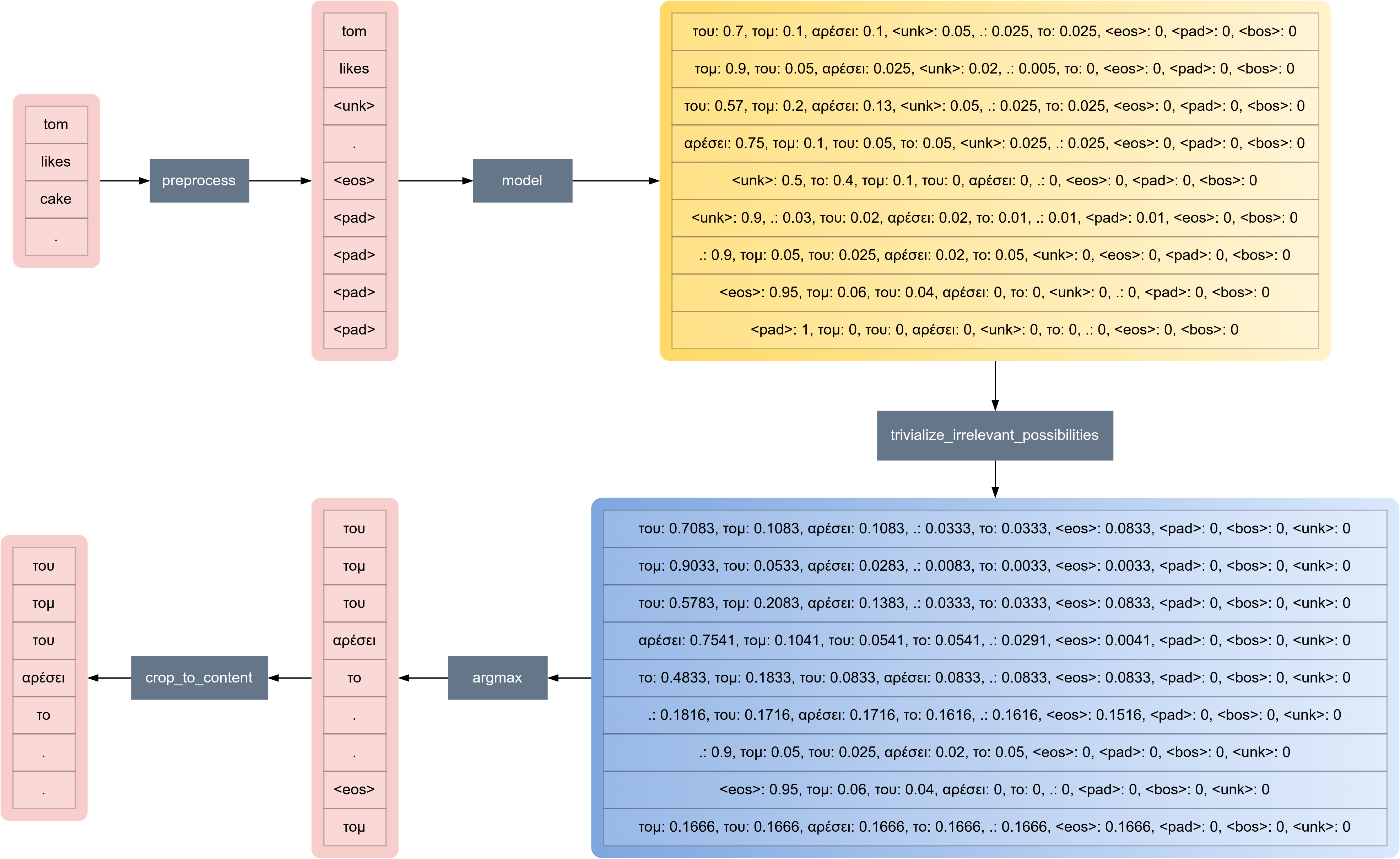
Moreover, during prediction time, after s2s_ell_pred generates a distribution, for each state, the probabilities of <unk>, <pad> and <bos>, are substituted by 0. Then the removed probability quantities are added up and distributed equally to the rest of the probabilities (see Figure 6). This is identical to the action of shrinking the sample space i.e. finding a conditional random variable. This is implemented in trivialize_irrelevant_possibilities located in the ./src/predictor.py file. Therefore even if <unk> has the highest probability after the model's output, no <unk> words will appear in the final target-token predictions, forcing the predictor to come up with some other token (except <pad> and <bos>) instead.

Figure 6. This is an example of how the predictor handles the output of a model that produces a distribution. The target's vocabulary is consisted of του, τομ, αρέσει, ., το, <eos>, <pad>, <bos>, <unk>.

Experimental Evaluation

For the evaluation of this model the two metrics that have been used were the loss function (categorical cross entropy), and a modified version of BLEU, which offered a much better insight to the quality of the model. The file containing the implementation of these metrics is ./src/metrics.py. The vectorized form of the loss function was defined in the following way. Select any of the dataset's ground truth distribution (or token in our case) $f$ and its estimation $\hat{f}$ infered by s2s_ell. $f$ and $\hat{f}$ are both rank 3 tensors where

• The first axis specifies the example denoted by $i$. The set where $i$ iterates on is a small minibatch sample.
• The second axis specifies the state's step, or the token's position inside the output sequence denoted by $j$.
• The third axis specifies the dimensionality of the output, coinciding with the target vocabularies size denoted by $k$.

Define $\mathcal{M}$ to be the rank 3 tensor having the same size as $f$, but where all its values are set to be $1$, except the positions where the final axis corresponds to <pad> where $\mathcal{M}$ is set to be $0$. To be precise, in the target language's vocabulary, the index of <pad> is $1$. Hence all values in $\mathcal{M}_{:,:,1}$ are set to $0$. $$\mathcal{L}(f,\hat{f}) = - \frac{400}{\sum \mathcal{M}} \cdot \sum \big( \mathcal{M} \odot \big( f \odot \log(\hat{f} + \epsilon) \big) \big)$$ $\epsilon$ is set to $10^{-20}$ and is used to prevent the function $\log$ from accepting the $0$ value, as distribution functions belong to the interval $[0,1]$ that includes $0$. Take the subset of 32 bit floating numbers that belong to that interval and we now have a finite set. This makes it likely that $0$ will be encountered in $\hat{f}$, during the training or even during predictions. That is why $\epsilon$ was added to $\hat{f}$. $\mathcal{M}$ is used to mask the tensor $f \odot \log(\hat{f} + \epsilon \big)$, because we don't want additional loss to be accumulated due to sequence positions where paddings should have been predicted at. In the above expression $\sum$ sums all its input-tensor's values.

BLEU on the other hand, is a metric that belongs in the interval $[0,1]$. This version of BLEU is specified in the following way. Suppose that for an example $i$ out of $m$ examples, $\text{len}^{(i)}$ is the length of the ground truth sequence $f$ starting from the first token, up to the token before the <eos> token, while $\text{len}_{\text{pred}}^{(i)}$ is the same kind of length but applied on the predicted sequence $\hat{f}$ instead. Drop all tokens after <eos> including that token too. Contruct collections of g-grams for all $g \in { 1, 2 }$. E.g.

Full sequence

Ground Truth: A E C D D E E F . <eos> <pad> <pad> <pad>
Prediction  : A G I . F E E F G H . <eos> <pad>

Trimmed to content

Ground Truth: A E C D D E E F .
Prediction  : A G I . F E E F G H .

1-grams collections

Ground Truth: ['A', 'E', 'C', 'D', 'D', 'E', 'E', 'F', '.']
Prediction  : ['A', 'G', 'I', '.', 'F', 'E', 'E', 'F', 'G', 'H', '.']

2-grams collection

Ground Truth: [('A', 'E'), ('E', 'C'), ('C', 'D'), ('D', 'D'), ('D', 'E'), ('E', 'E'), ('E', 'F'), ('F', '.')]
Prediction  : [('A', 'G'), ('G', 'I'), ('I', '.'), ('.', 'F'), ('F', 'E'), ('E', 'E'), ('E', 'F'), ('F', 'G'), ('G', 'H'), ('H', '.')]

From the two lists of 1-grams, the common tokens are

['A', 'E', 'F', '.']

while for the 2-grams we get

[('E', 'E'), ('E', 'F')]

What what do now is that for every common 1-gram, count the number of 1-gram repetitions for both the ground truth and prediction. We have

1-grams	'A'	'E'	'F'	'.'
ground truth	1	3	1	1
prediction	1	2	1	2
min	1	2	1	1

The same is done for 2-grams

2-grams	('E', 'E')	('E', 'F')
ground truth	1	1
prediction	1	1
min	1	1

For every gram size $g$ (either $1$ or $2$), define $p_g^{(i)}$ to be the corresponding table's row summed and divided by the length of the associated collection of the prediction's $g$-gram. We get $$p_1^{(i)} = \frac{1+2+1+1}{11} = \frac{6}{11}, \ \ \ \ \ \ p_2^{(i)} = \frac{1+1}{10} = \frac{2}{10}.$$

Now BLEU is computed as $$\text{BLEU} = \frac{1}{m} \cdot \sum_{i=0}^{m-1} \bigg( \exp \bigg( \min \bigg( \bigg \{ 0, 1- \frac{\text{len}^{(i)}}{\text{len}^{(i)}_{\text{pred}}} \bigg \} \bigg) \bigg) \cdot \prod_{g=1}^{2} (p_g^{(i)})^{1/2^g} \bigg).$$

BLEU was implemented in a way so that it does not take into account the <unk> token. Hence if <unk> exists inside any $g$-gram, that $g$-gram will not contribute to the score at all. The higher the BLEU of two sequences, the more identical they are. If two sequences are exactly the same, then BLEU will equal $1$ for that specific example. The exponent of $p_g^{(i)}$ in the above relation, "weights" $p_g^{(i)}$ more when $g$ is increased.

Now that the metrics were defined, we can proceed with the description of the training/experiment. The results of this training (see Figure 7) are certainly interesting, however it has to be admitted that s2s_ell does not apply that well to external data.

During the training, the two metrics were computed on both the teacher forcing (Figure 4) and predictor (Figure 5) implementations of s2s_ell.

Sample from the training set:

    [eng]                                      [ell]
0   we were all tired .                        ήμαστε όλοι κουρασμένοι .
1   what's living in boston like ?             πως είναι να ζεις στη βωστόνη ;
2   my hobby is collecting old <unk> .         το χόμπι μου είναι να συλλογή να το
3   europe is a <unk> .                        η ευρώπη είναι μια .
4   everyone was drunk .                       όλοι ήταν πιωμένοι .
5   when i return , we'll talk .               όταν επιστρέψω , θα μιλήσουμε .
6   they wanted to steal the car .             θέλησαν να κλέψουν τ' αμάξι .
7   did you buy flowers ?                      αγόρασες λουλούδια ;
8   who are you ?                              ποιος είσαι ;
9   i doubt if it would be fun to              αμφιβάλλω αν θα ήταν διασκεδαστικό να το κάνεις

Sample from the validation set:

    [eng]                                      [ell]
0   your car's ready .                         το αυτοκίνητό σου είναι έτοιμο .
1   tom moved to australia .                   ο τομ είν' στην αυστραλία στην .
2   i'll find them .                           θα τα βρω .
3   does this count ?                          μετράει αυτό ;
4   i don't understand this .                  δεν καταλαβαίνω αυτό .
5   tom has trouble talking to girls .         ο τομ δυσκολεύεται να μιλήσει σε κορίτσια .
6   i was proud of you .                       ήμουν περήφανη για σας .
7   is tom married ?                           ο τομ είναι παντρεμένος ;
8   give us three minutes .                    δώστε μας τρία λεπτά .
9   <unk> are starting again soon .            οι άνδρες είναι ο βραβείο .

Judging by the sample provided above, all example sources that include the <unk> token, correspond to problematic target translations as expected. Validation example #9 has the worst translation from all the rest in this sample. This is logical, as <unk> is the first token of the source sequence and the only one with so many state-steps behind, when compared to all other examples. Hence, it is far easier for the translator to lose control and hallucinate. All future tokens are affected by it, giving absolutely no guidance or information about the proper context of the input sequence.

The model is observed to be stable in cases where the source's <unk> is close to the end. Training example #3 is an indication of that stability.

Maybe the model overfits or maybe not. We can't be sure by looking at these examples only. That's where the final model's metrics come in.

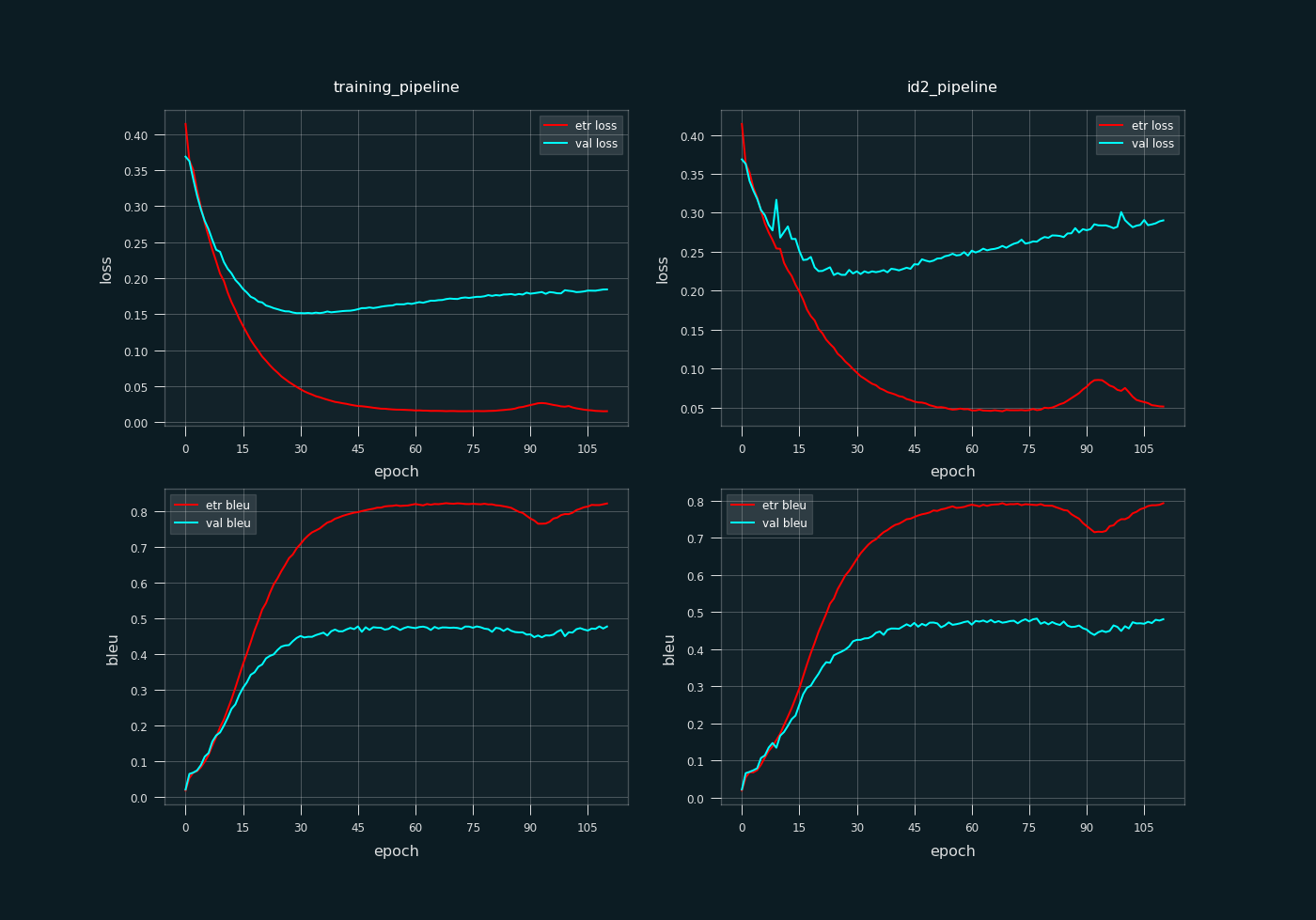
Figure 7. Evaluation metrics on both the training pipeline (training_pipeline = s2s_ell_train) as seen on the left column, and on the prediction pipeline (id2_pipeline = s2s_ell_pred) as seen on the right column. loss refers to the categorical cross entropy loss function, and bleu is our implementation of the BLEU metric. etr <metric> refers to the minibatch-wise <metric> measurement on the training set, while val <metric> is a measurement of <metric> on the validation set, where <metric> is either loss or bleu.

The optimal model was selected with respect to the BLEU metric of s2s_ell_pred on the validation set, with the highest value produced on epoch 77, just before the model passed through a local spike (noticeable between epoch 75 and 105). The training's path is ./training/ell/s2s_ell.pt

Current translator's evaluation on the training pipeline s2s_ell_train (teacher forcing)

s2s_ell_train	training set	validation set
loss	0.015187	0.173969
bleu	0.820327	0.475963

and on the prediction pipeline s2s_ell_pred

s2s_ell_pred	training set	validation set
loss	0.046581	0.262963
bleu	0.788092	0.481982

Comparing the BLEU metric between the training and validation set (see Figure 7), the model obviously shows an overfitting trend. Both metrics differ a lot, in both pipelines. Also no significant exposure bias is indicated by the training, as the performance difference between s2s_ell_pred and s2s_ell_train is not that significant. BLEU metrics seem to converge on a value close to 0.475, discouraging to add more epochs for the training.

Setup

Linux Terminal

The computer is required to be equipped with an NVIDIA GPU with Cuda installed on its OS. To verify you have Cuda installed you expect

nvidia-smi

to return something like this

Sun Mar 26 17:33:25 2023       
+-----------------------------------------------------------------------------+
| NVIDIA-SMI 525.85.12    Driver Version: 525.85.12    CUDA Version: 12.0     |
|-------------------------------+----------------------+----------------------+
| GPU  Name        Persistence-M| Bus-Id        Disp.A | Volatile Uncorr. ECC |
| Fan  Temp  Perf  Pwr:Usage/Cap|         Memory-Usage | GPU-Util  Compute M. |
|                               |                      |               MIG M. |
|===============================+======================+======================|
|   0  Tesla T4            Off  | 00000000:00:04.0 Off |                    0 |
| N/A   43C    P8    10W /  70W |      0MiB / 15360MiB |      0%      Default |
|                               |                      |                  N/A |
+-------------------------------+----------------------+----------------------+
                                                                               
+-----------------------------------------------------------------------------+
| Processes:                                                                  |
|  GPU   GI   CI        PID   Type   Process name                  GPU Memory |
|        ID   ID                                                   Usage      |
|=============================================================================|
|  No running processes found                                                 |
+-----------------------------------------------------------------------------+

Now, open a Linux terminal, navigate to machine_translator/src and execute

!gcc ./preprocessing_tools.c -o ./lib/preprocessing_tools.so -shared

The cool looking dark theme pip package is ing_theme_matplotlib.

To train a model use

python3 train.py

This saves the trainings in .pt format, storing them inside machine_translator/training. By default, this trains a model from scratch. To parse that file and continue training on its respective model, open the file train.py, replace the last two lines

train_from_scratch(device=device)
# load_and_train_model(training_path=<path_to_training>, device=device)

with

# train_from_scratch(device=device)
load_and_train_model(training_path=<path_to_training>, device=device)

To predict on a model (e.g. the demo s2s_ell), execute

python3 predict.py

Jupyter Notebook

One way to make the Jupyter Notebook functional in a google colab environment in GPU runtime:

1. Create the following google drive directory hierarchy

MyDrive [Google drive's uppermost directory]
   |---Colab Notebooks [.ipynb files]
   |
   |---colab_storage
                |---datasets
                |---scripts [.c files]
                |---lib [.so files]
                |---training

2. Copy ./src/machine_translator.ipynb from this repository to the google drive's directory MyDrive/Colab Notebooks.
3. Copy ./src/preprocessing_tools.c to MyDrive/colab_storage/scripts.

After you create this hierarchy and copy the files, the rest is up to the jupyter kernel. Note that the first executable snippet

from google.colab import drive
drive.mount('/content/drive')

will ask for permission to access your google drive's directories. Give that access to google colab to invoke that hierarchy. The reason this was set up this way is to make the files persistent, and not runtime-dependent.

Training Checkpoints

During training, the models and information about their trainings are systematically saved inside ./training, stored in a .pt file. For every epoch, an image file named as

<model_name>_live.png

shows the evaluation metrics' plots of the model throughout all past epochs. Also, the .pt file, when parsed through torch's load method, the resulting variable is a dictionary containing the following items:

'model_params': <`torch.nn.Module.state_dict()` containing the model's architecture and trainable parameters.>,
'src_vocab': <Type: `torchtext.vocab`. Source vocabulary.>,
'src_vocab_size': <Type: `int`. Source vocabularies size.>,
'tgt_vocab': <Type: `torchtext.vocab`. Target vocabulary.>,
'tgt_vocab_size': <Type: `int`. Target vocabularies size.>,
'max_steps_src': <Type: `int`. Padded source sequence's number of steps.>,
'max_steps_tgt': <Type: `int`. Padded target sequence's number of steps.>,
'data_info':
{
    'n_train': <Type: `int`. Size of training set.>,
    'n_val': <Type: `int`. Size of validation set.>
},
'metrics_history':
{
    'loss':
    {
        'training_pipeline':
        {
            'train': <Type: `list`. Loss history of training pipeline measured on the training set.>,
            'val': <Type: `list`. Loss history of training pipeline measured on the validation set.>
        },
        'id2_pipeline':
        {
            'train': <Type: `list`. Loss history of the prediction pipeline, measured on the training set.>,
            'val': <Type: `list`. Loss history of the prediction pipeline, measured on the validation set.>
        }
    },
    'bleu':
    {
        'training_pipeline':
        {
            'train': <Type: `list`. BLEU history of training pipeline measured on the training set.>,
            'val': <Type: `list`. BLEU history of training pipeline measured on the validation set.>
        },
        'id2_pipeline':
        {
            'train': <Type: `list`. BLEU history of the prediction pipeline, measured on the training set.>,
            'val': <Type: `list`. BLEU history of the prediction pipeline, measured on the validation set.>
        }
    }
},
'training_hparams':
{
    'epoch': <Type: `int`. Current epoch.>,
    'learning_rate': <Type: `float`. Learning rate.>,
    'minibatch_size': <Type: `int`. Minibatch size.>
},
'delta_t': <Type: `float`. Total time (in seconds) taken to complete training.>,
'shuffle_seed': <Type: `int`. Seed for the data shuffling RNG.>,
'dataset_name': <Type: `str`. Name of dataset.>

The reason that torch.nn.Module.state_dict() was prefered to be stored in the .pt file instead of model itself, was to allow model information to be parsed in different machines without worrying about deserialization errors due to CUDA or PyTorch version incompatibilies.

For a given epoch, its training state may be saved inside ./training under the following circumstances.

• The current training pipeline's BLEU measured on the validation set surpasses all its past values. Filename format

<model_name>_opt.pt

• The current epoch belongs to the trainer's attribute scheduled_checkpoints. These checkpoints are persistent and won't be deleted in the following epochs. Filename format

<model_name>_ep<epoch>.pt

• Depending on the trainer's backup frequency attribute bkp_freq. Filename format

<model_name>_live_ep<epoch>.pt

Experimental Conclusion and Software Improvements

It seems like an increased minibatch size leads to better trainings and faster convergence. The <unk> token should not be that frequently encountered, and especially in sequences where it is located close to the start. Also, allowing wider sequences with more tokens is definitely a way to increase performance. Any kind of regularization technique used, like dropout, did more harm than good to the final model's performance, that is why we did not implement s2s_ell using dropout.

A critical factor to consider when judging the preceding results, is that the validation set is not a good enough representation of external data. One may argue that the training vs validation set split is random, and thus we cannot know that. However by looking at the dataset, it is almost certain that the validation set is composed of data identical to the training set, making it a biased set, unable to provide us with enough information to evaluate the model's ability to generalize. As a consequence, the real overfitting is definitely way worse than the one implied by the metrics' differences between the two sets.

It all comes down to the dataset's size. Perhaps 5000000 examples would suffice. The selection of validation examples has to be selected randomly, and independently of the training set. Also in large datasets one would need a lot of memory and the training is obviously expected to take a lot longer.