cnn-transfer-learning

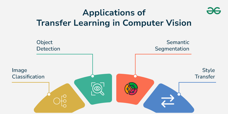
Image Credit to Explain the concept of transfer learning and its application in computer vision

Accelerating Shape Classification with Transfer Learning

In the previous post, we delved into the creation of a Convolutional Neural Network (CNN) from scratch to classify geometric shapes. While this approach is a valuable learning exercise, it may not always be the most efficient, especially when dealing with larger, more complex datasets or when computational resources are limited. This is where transfer learning comes into play. In this post, we’ll explore how transfer learning can supercharge our shape classification tasks and any other image recognition projects.

What is Transfer Learning?

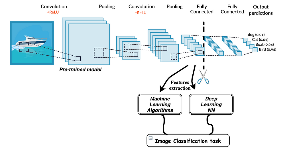
Image Credit to Transfer Learning for Image Classification in PyTorch

Transfer learning is a machine learning strategy where a model trained on one task is repurposed on a related task. It's like applying knowledge learned from one subject to another subject in school. This technique can drastically reduce the amount of training data and computational resources required, making it a powerful tool in the machine learning toolbox.

For instance, consider a CNN model pre-trained on ImageNet, a large dataset containing millions of images across thousands of categories. The lower layers of this model have already learned to detect fundamental features like edges, textures, and patterns. By leveraging these pre-learned features and only fine-tuning the upper layers to classify shapes, we can adapt the model for our specific task without retraining the entire network.

Perception in Neural Network Training and Transfer Learning

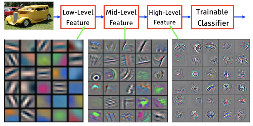
Image Credit to Transfer Learning for Image Classification in PyTorch

Perception, the process of interpreting input data, is crucial in training neural networks. When training from scratch, a model must learn to perceive features and patterns, which can be time-consuming and computationally intensive.

Transfer learning accelerates this process by leveraging the perception learned by a pre-trained model. This reduces the need for extensive training and resources, as the model doesn't need to learn perception from scratch. Instead, it focuses on the specific features relevant to the new task, leading to faster training times and potentially improved performance.

In essence, transfer learning facilitates quicker experimentation and innovation in machine learning by building on pre-learned perception.

Understanding the Foundations of Perception

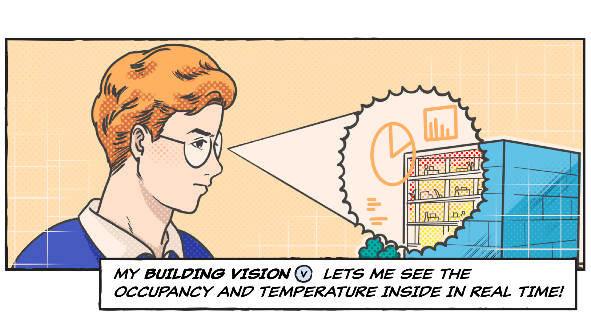
Image Credit to Perception! Immersion! Empowerment! Superpowers as Inspiration for Visualization

The initial layers of a CNN trained for Shape Classification have learned to extract the fundamental building blocks of visual perception. These layers act as feature extractors, identifying and encoding low-level features such as:

• Edges: The boundaries between different regions in an image.
• Textures: The patterns or structures within regions.
• Shapes: The geometric outlines of objects.
• Colors: The hue, saturation, and brightness of pixels.

Perception: A Philosophical View

Perception, in its broadest sense, refers to the process of becoming aware or conscious of something through the senses. It's a cognitive process that allows us to interpret our surroundings using the data we collect through our senses. Philosophically, perception is a complex process involving various stages and components, and it's the primary means through which we experience the world.

When we see an object, hear a sound, touch a surface, our senses collect raw, unprocessed data. This data is then interpreted by our brain, which recognizes patterns, compares them to previous experiences, and constructs a coherent representation of our environment. This entire process is perception.

Perception in Machine Learning

When we talk about perception in the context of machine learning, particularly deep learning, we're referring to a model's ability to "understand" or "interpret" input data. In the case of a Convolutional Neural Network (CNN) used for image recognition, the initial layers of the network learn to perceive fundamental visual features such as edges, textures, and colors. As we move deeper into the network, the layers learn to recognize more complex patterns and structures.

In the early layers of a CNN, the model learns low-level features (edges, colors, textures), similar to how our eyes first perceive these basic elements in our visual field. As the information moves through the network (or our brain), these low-level features are combined and recombined to form higher-level features (shapes, patterns), and eventually objects that we can recognize.

Leveraging Pre-trained Knowledge

Consider a pre-trained CNN model on ImageNet, a massive dataset with millions of images across various categories. The initial layers in this model have already learned to identify fundamental features like edges, textures, and patterns.

By leveraging these pre-learned features, we can fine-tune the upper layers to classify shapes. This allows us to adapt the model for our specific task without retraining the entire network from scratch.

The Computational Benefits

Training a deep neural network from scratch can be computationally expensive, especially when dealing with large datasets or complex models. Using pre-trained layers can offer significant computational savings:

• Reduced Training Time: As mentioned above, training the upper layers is much faster than training the entire network from scratch.
• Lower Hardware Requirements: Smaller models or lower-resolution images can be used, reducing the computational demands on hardware.
• Energy Efficiency: Less computational work means less energy consumption.

Why Use Transfer Learning for Shape Classification?

Transfer learning brings several benefits to the table, especially for tasks involving simple or synthetic data like shape classification:

1. Efficiency: Pre-trained models already know how to detect general patterns, such as edges or curves, which are crucial for identifying shapes. Instead of training a model from scratch, we fine-tune an existing model, saving time and computational resources.

2. Improved Accuracy: Pre-trained models have often been trained on large, diverse datasets, making them more robust in identifying features that our task-specific dataset might not cover comprehensively.

3. Faster Convergence: Since the model is starting with weights that already work for similar tasks, the learning process converges much faster than when initializing random weights.

Potential Applications of Transfer Learning

Transfer learning has found applications in a wide range of fields:

1. Computer Vision: Transfer learning is widely used in image classification, object detection, and image segmentation tasks. Pre-trained models like VGG16, ResNet, and Inception have been trained on large image datasets like ImageNet and can be fine-tuned for specific tasks with much less data.

2. Natural Language Processing (NLP): In NLP, models like BERT, GPT-2, and RoBERTa, trained on massive text corpora, are used as a starting point for tasks like sentiment analysis, text classification, and named entity recognition.

3. Medical Imaging: In healthcare, transfer learning is used to analyze medical images with high accuracy. Pre-trained models can be fine-tuned to detect and classify diseases in X-rays, MRIs, and CT scans, even when the available medical image dataset is small.

4. Autonomous Vehicles: Transfer learning is used in autonomous driving for tasks like object detection, semantic segmentation, and behavior cloning. Pre-trained models can be fine-tuned to adapt to different driving conditions and environments.

A Step-by-Step Guide to Transfer Learning

Now, let's dive into a practical example. We'll use PyTorch, a popular deep learning library, and PyTorch Lightning, a high-level interface for PyTorch, to demonstrate transfer learning in a simple image classification task.

1. Defining the Base Model: The SimpleShapeClassifier class defines a simple Convolutional Neural Network (CNN) model for shape classification. It includes methods for the forward pass, training, validation, testing, and configuring optimizers. This model is trained on a dataset of images with shapes like circles, squares, and triangles.

2. Creating a New Dataset: The script introduces new shapes (star, pentagon) and generates images for these new shapes using the generate_new_shape_image function. It then creates a new dataset, splits it into training and validation sets, and creates data loaders.

3. Transfer Learning for New Shapes: The TransferShapeClassifier class extends the SimpleShapeClassifier class. It freezes the convolutional layers and replaces the last fully connected layer to match the number of classes in the new dataset. This is the essence of transfer learning - reusing the lower layers of the model that have learned to detect fundamental features like edges and textures, and fine-tuning the upper layers to classify new shapes.

   class TransferShapeClassifier(SimpleShapeClassifier):
       def __init__(self, num_classes, learning_rate=0.001):
           super().__init__(num_classes, learning_rate)
           # Freeze the convolutional layers
           for param in self.conv1.parameters():
               param.requires_grad = False
           for param in self.conv2.parameters():
               param.requires_grad = False
           # Replace the last fully connected layer to match the number of classes in the new dataset
           self.fc2 = torch.nn.Linear(128, num_classes)

4. Training and Testing the New Model: The script trains the new model on the new dataset and tests it. This is done using the PyTorch Lightning's Trainer class, which simplifies the training process.

   # Define new model
   new_model = TransferShapeClassifier(num_classes=len(NEW_SHAPES))
   
   # Define new trainer
   new_trainer = pl.Trainer(max_epochs=10, default_root_dir='./logs')
   
   # Train new model
   new_trainer.fit(new_model, new_train_loader, new_val_loader)
   
   # Test new model
   new_test_dataset = torch.utils.data.TensorDataset(new_dataset, new_labels)
   new_test_loader = DataLoader(new_test_dataset, batch_size=32, shuffle=False)
   new_trainer.test(model=new_model, dataloaders=new_test_loader)

5. Predicting Shapes for New Unseen and Seen Images: The script generates new unseen and seen images and uses the new model to predict their shapes. This demonstrates the effectiveness of the transfer learning approach.

   # Predict shape for new unseen image
   print("Generating new image [unseen shape = hexagon]")
   new_image_unseen = generate_new_shape_image('hexagon')
   predicted_shape = predict_shape(new_model, new_image_unseen, NEW_SHAPES)
   print(f"Predicted shape: {predicted_shape}")
   
   # Predict shape for new seen image
   print("Generating new image [seen shape = star]")
   new_image_seen = generate_new_shape_image('star')
   predicted_shape = predict_shape(new_model, new_image_seen, NEW_SHAPES)
   print(f"Predicted shape: {predicted_shape}")
   print("Generating new image [seen shape = pentagon]")
   new_image_seen = generate_new_shape_image('pentagon')
   predicted_shape = predict_shape(new_model, new_image_seen, NEW_SHAPES)
   print(f"Predicted shape: {predicted_shape}")

This script demonstrates how transfer learning can be used to adapt a model trained on one task (classifying certain shapes) to a related task (classifying new shapes), saving computational resources and improving efficiency.

Output

/Library/Frameworks/Python.framework/Versions/3.10/lib/python3.10/site-packages/transformers/utils/generic.py:441: FutureWarning: `torch.utils._pytree._register_pytree_node` is deprecated. Please use `torch.utils._pytree.register_pytree_node` instead.
  _torch_pytree._register_pytree_node(
GPU available: True (mps), used: True
TPU available: False, using: 0 TPU cores
HPU available: False, using: 0 HPUs

  | Name    | Type      | Params | Mode 
----------------------------------------------
0 | conv1   | Conv2d    | 896    | train
1 | conv2   | Conv2d    | 18.5 K | train
2 | pool    | MaxPool2d | 0      | train
3 | dropout | Dropout   | 0      | train
4 | fc1     | Linear    | 33.6 M | train
5 | fc2     | Linear    | 258    | train
6 | relu    | ReLU      | 0      | train
----------------------------------------------
33.6 M    Trainable params
0         Non-trainable params
33.6 M    Total params
134.297   Total estimated model params size (MB)
7         Modules in train mode
0         Modules in eval mode
Sanity Checking: |                                        | 0/? [00:00<?, ?it/s]/Library/Frameworks/Python.framework/Versions/3.10/lib/python3.10/site-packages/pytorch_lightning/trainer/connectors/data_connector.py:424: The 'val_dataloader' does not have many workers which may be a bottleneck. Consider increasing the value of the `num_workers` argument` to `num_workers=9` in the `DataLoader` to improve performance.
/Library/Frameworks/Python.framework/Versions/3.10/lib/python3.10/site-packages/pytorch_lightning/trainer/connectors/data_connector.py:424: The 'train_dataloader' does not have many workers which may be a bottleneck. Consider increasing the value of the `num_workers` argument` to `num_workers=9` in the `DataLoader` to improve performance.
/Library/Frameworks/Python.framework/Versions/3.10/lib/python3.10/site-packages/pytorch_lightning/loops/fit_loop.py:298: The number of training batches (25) is smaller than the logging interval Trainer(log_every_n_steps=50). Set a lower value for log_every_n_steps if you want to see logs for the training epoch.
Epoch 9: 100%|████████████████████████| 25/25 [00:01<00:00, 16.89it/s, v_num=23]`Trainer.fit` stopped: `max_epochs=10` reached.                                 
Epoch 9: 100%|████████████████████████| 25/25 [00:01<00:00, 13.89it/s, v_num=23]
/Library/Frameworks/Python.framework/Versions/3.10/lib/python3.10/site-packages/pytorch_lightning/trainer/connectors/data_connector.py:424: The 'test_dataloader' does not have many workers which may be a bottleneck. Consider increasing the value of the `num_workers` argument` to `num_workers=9` in the `DataLoader` to improve performance.
Testing DataLoader 0: 100%|█████████████████████| 32/32 [00:00<00:00, 69.55it/s]
┏━━━━━━━━━━━━━━━━━━━━━━━━━━━┳━━━━━━━━━━━━━━━━━━━━━━━━━━━┓
┃        Test metric        ┃       DataLoader 0        ┃
┡━━━━━━━━━━━━━━━━━━━━━━━━━━━╇━━━━━━━━━━━━━━━━━━━━━━━━━━━┩
│         test_loss         │    0.02593466266989708    │
└───────────────────────────┴───────────────────────────┘
Generating new image [unseen shape = circle]
Predicted shape: triangle
Generating new image [seen shape = triangle]
Predicted shape: triangle
GPU available: True (mps), used: True
TPU available: False, using: 0 TPU cores
HPU available: False, using: 0 HPUs

  | Name    | Type      | Params | Mode 
----------------------------------------------
0 | conv1   | Conv2d    | 896    | train
1 | conv2   | Conv2d    | 18.5 K | train
2 | pool    | MaxPool2d | 0      | train
3 | dropout | Dropout   | 0      | train
4 | fc1     | Linear    | 33.6 M | train
5 | fc2     | Linear    | 258    | train
6 | relu    | ReLU      | 0      | train
----------------------------------------------
33.6 M    Trainable params
19.4 K    Non-trainable params
33.6 M    Total params
134.297   Total estimated model params size (MB)
7         Modules in train mode
0         Modules in eval mode
Epoch 9: 100%|████████████████████████| 25/25 [00:00<00:00, 26.51it/s, v_num=24]`Trainer.fit` stopped: `max_epochs=10` reached.                                 
Epoch 9: 100%|████████████████████████| 25/25 [00:01<00:00, 19.86it/s, v_num=24]
Testing DataLoader 0: 100%|█████████████████████| 32/32 [00:00<00:00, 68.57it/s]
┏━━━━━━━━━━━━━━━━━━━━━━━━━━━┳━━━━━━━━━━━━━━━━━━━━━━━━━━━┓
┃        Test metric        ┃       DataLoader 0        ┃
┡━━━━━━━━━━━━━━━━━━━━━━━━━━━╇━━━━━━━━━━━━━━━━━━━━━━━━━━━┩
│         test_loss         │   0.008498326875269413    │
└───────────────────────────┴───────────────────────────┘
Generating new image [unseen shape = hexagon]
Predicted shape: star
Generating new image [seen shape = star]
Predicted shape: star
Generating new image [seen shape = pentagon]
Predicted shape: pentagon

Evaluating Transfer Learning: A Closer Look at Test Loss

When we train machine learning models, one of the most critical aspects is evaluating their performance. This is particularly important in transfer learning, where we repurpose a pre-trained model on a new task. One common metric used for this purpose is the test loss. In this section, we'll delve into what test loss is, why it's important, and things to consider when interpreting it in the context of transfer learning.

Understanding Test Loss

Test loss is a measure of how well a model performs on the test dataset, which is data that the model has not seen during training. It's calculated by applying the model to the test data and comparing the model's predictions to the actual values using a loss function. In classification problems, a common loss function used is cross-entropy loss.

A lower test loss indicates that the model's predictions are close to the actual values, suggesting that the model is performing well on the test dataset. Conversely, a high test loss suggests that the model's predictions are far from the actual values, indicating poor performance.

Test Loss in Transfer Learning

In transfer learning, we leverage the knowledge from a pre-trained model to improve performance on a new task. The test loss can provide valuable insights into how well this process is working.

For instance, if the test loss of the transfer learning model is significantly lower than that of a model trained from scratch, this suggests that transfer learning has successfully leveraged the knowledge from the original task to improve performance on the new task.

Things to Consider

While test loss is a useful metric, it's important to consider the following points when interpreting it:

1. Other Performance Metrics: Test loss is not the only measure of a model's performance. Other metrics like accuracy, precision, recall, and F1 score should also be considered, especially for imbalanced datasets. These metrics can provide a more comprehensive view of the model's performance.

2. Overfitting: A low test loss is generally a good sign, but it's crucial to ensure that the model is not overfitting to the training data. Overfitting occurs when a model learns the training data too well, to the point where it performs poorly on unseen data. Techniques like cross-validation, regularization, and dropout can help prevent overfitting.

3. Underfitting: On the other hand, if the test loss is too high, it might be a sign that the model is underfitting. Underfitting occurs when a model is too simple to capture the complexity of the data. In this case, a more complex model or more training might be needed.

4. Data Quality: The quality of the test data can also impact the test loss. If the test data is noisy, contains errors, or is not representative of the real-world data the model will encounter, the test loss may not provide an accurate measure of the model's performance.

Test loss is a valuable metric in evaluating the performance of transfer learning models. However, it should be interpreted in the context of other performance metrics, and considerations should be made for overfitting, underfitting, and data quality. By doing so, we can gain a more comprehensive understanding of our model's performance and make more informed decisions in our machine learning projects.

Troubleshooting Common Issues

Here are some common issues you might encounter when using transfer learning and how to address them:

• High Test Loss:

  • Check Task Similarity: Ensure that the new task is closely related to the original task.
  • Increase Fine-Tuning: If the task is less related, try fine-tuning more layers or training some layers from scratch.
  • Improve Data Quality: Look for noise, outliers, or biases in your data.
  • Adjust Hyperparameters: Experiment with different hyperparameters, such as learning rate or batch size.

• Overfitting:

  • Regularization: Use techniques like L1 or L2 regularization to prevent overfitting.
  • Data Augmentation: Increase the diversity of your training data to reduce overfitting.
  • Early Stopping: Stop training when the validation loss starts to increase.

• Underfitting:

  • Increase Model Complexity: Try using a larger pre-trained model or adding more layers.
  • Increase Training Time: Train the model for longer.
  • Improve Data Quality: Ensure that your data is representative of the task.

• Convergence Issues:

  • Adjust Learning Rate: Experiment with different learning rates.
  • Check Gradient Explosions/Vanishing Gradients: Use techniques like gradient clipping or normalization.
  • Consider Batch Normalization: Batch normalization can help stabilize training.

By understanding the factors that influence test loss and addressing common troubleshooting issues, you can effectively leverage transfer learning to improve the performance of your machine learning models.

Transfer Learning and Large Language Models

By leveraging the knowledge encoded in the pre-trained model, you can significantly reduce training time and improve performance, especially when dealing with limited datasets.

• Knowledge Transfer: LLMs, such as LLaMA, GPT, and BERT, have learned to understand language structure, semantics, and context from their massive pre-training datasets. Fine-tuning leverages this knowledge to quickly adapt to new tasks.
• Efficiency: Fine-tuning often requires less training data and time compared to training a model from scratch. This is particularly beneficial when dealing with limited resources or time constraints.
• Improved Performance: The pre-trained model's knowledge can provide a strong foundation, leading to better performance on downstream tasks.

Fine-Tuning LLMs: A Step-by-Step Approach

The process of fine-tuning an LLM involves several key steps:

1. Obtain the Pre-trained Model: Download the desired LLM model from the appropriate repository.
2. Prepare Your Dataset: Create a dataset that is representative of the task you want to fine-tune the model for. Ensure the data is cleaned, formatted, etc.
3. Define the Fine-Tuning Parameters: Set parameters like the learning rate, batch size, and number of epochs.
4. Train the Model: Feed your dataset to the pre-trained LLM and train it. The model will adjust its parameters to better fit the specific task.
5. Evaluate the Model: Use a validation set to assess the model's performance during training and adjust parameters as needed.

The Versatility of Fine-Tuned LLMs

Fine-tuned LLMs have a wide range of applications, including:

• Question Answering: Answering questions based on provided text or knowledge bases.
• Text Summarization: Condensing long texts into shorter summaries.
• Translation: Translating text from one language to another.
• Creative Writing: Generating creative text formats like poems, stories, or scripts.
• Code Generation: Assisting developers in writing code.

Limitations of Transfer Learning

Transfer Learning: A Double-Edged Sword

While transfer learning offers significant benefits, it's not a silver bullet. Its effectiveness hinges on several factors:

• Domain Alignment: The closer the pre-trained model's task is to yours, the more likely it is to transfer useful knowledge. A model trained on cat images might struggle with recognizing cars, highlighting the importance of domain alignment.
• Overreliance on Pre-trained Features: Relying too heavily on pre-trained features can limit your model's ability to learn unique patterns specific to your task. Striking a balance between leveraging pre-trained knowledge and allowing the model to learn new features is crucial.
• Bias Amplification: Pre-trained models can inherit biases present in their training data. If the original dataset was biased, the transferred model might perpetuate those biases, leading to unfair or inaccurate predictions.

Internet Scraping: A Data Minefield

Internet scraping, while a tempting source of data, comes with significant risks:

• Legal Quagmire: Scraping websites without explicit permission can violate terms of service and potentially lead to legal consequences. Always respect website owners' rights and adhere to legal guidelines.
• Ethical Dilemmas: Scraping personal data raises privacy concerns and can violate individuals' rights. Handle personal information responsibly and ethically.
• Data Quality Concerns: Scraped data can be noisy, incomplete, or biased, affecting your model's performance. Clean and preprocess scraped data carefully to ensure its quality.
• Website Restrictions: Many websites implement measures to prevent scraping, such as CAPTCHAs or rate limiting. These can make data collection challenging.

Bias in Machine Learning

Bias in machine learning arises when a model's predictions are systematically skewed towards a particular group or outcome. This can be due to several factors:

• Biased Data: If the training data is biased, the model will likely learn to perpetuate those biases. For instance, a model trained on a dataset with predominantly white faces may struggle to recognize faces of people with darker skin tones.
• Biased Algorithms: Some algorithms may be more susceptible to bias amplification than others. Careful algorithm selection is essential.
• Human Bias: Human biases can creep into the design and implementation of machine learning models. Developers must be mindful of their own biases and strive for objectivity.

Mitigating These Challenges

To address these limitations and challenges, consider the following strategies:

• Data Quality and Diversity: Ensure your training data is diverse, representative, and free from biases.
• Algorithm Selection: Choose algorithms known for their robustness to bias.
• Bias Detection and Mitigation: Employ techniques to identify and address biases in your models.
• Ethical Considerations: Prioritize ethical practices in data collection and usage.
• Alternative Data Sources: Explore alternative sources like public datasets, surveys, or synthetic data generation.

By carefully navigating these challenges, you can harness the power of transfer learning and internet scraping while minimizing their risks.

Conclusion

Transfer learning is a powerful technique that enables the efficient adaptation of neural networks to various tasks. By leveraging the knowledge encoded in pre-trained models, you can achieve impressive results, even with limited datasets.