Discovering Themes in Text with Topic Modeling (Latent Dirichlet Allocation)

Description

The method uncovers frequently discussed topics (or themes) in a document collection. The topics are represented by their most prominent words. These topics allow to explore document collections or can be used as labels in subsequent tasks. For example, applying the method to a hotel reviews corpus may result in topics that represent room quality, food quality, pricing, and so on, with each review being linked to the respective topics. In technical terms, it calculates the co-occurrence frequencies of words in documents to organize documents as distribution of topics and topics as distribution of words. The method reads input as a document per line and outputs two files, containing the document-topic distribution and topic-word distribution respectively.

Use Cases

Exploring the main topics discussed in a social media corpus for different user groups (e.g., different demographics). One can use each social media post as a document and use this method to compute the document-topic distribution. Then use information on to which group the posting user for each post belongs to get an average topic distribution for the different user groups. Then have a look at the topic-word distribution to name each topic (e.g., health care, immigration, the economy, etc.) and use the average topic distribution to see the different interests of the different user groups.

Input Data

This methods takes as input a text file with one document per line. For example, BBC news article headlines as in data/input-data/news-headings.txt:

India calls for fair trade rules
Sluggish economy hits German jobs
Indonesians face fuel price rise
Court rejects $280bn tobacco case
Dollar gains on Greenspan speech
...

Output Data

This method produces the document-topic distribution and topic-word distribution as two separate TSV files (Tab-Separated Values).

Each row in the document-topic distribution file shows for a document (respective line in the input file) the topic distribution and the document text. For the example above and three topics, the output is as in data/output-data/document-topic-distribution.tsv (e.g., the topics of the first document are 37.5% topic 1, 25.0% topic 2, and 37.5% topic 3):

topic-1	topic-2	topic-3	Text
0.375	0.25	0.375	India calls for fair trade rules
0.375	0.25	0.375	Sluggish economy hits German jobs
0.375	0.25	0.375	Indonesians face fuel price rise
0.375	0.375	0.25	Court rejects $280bn tobacco case
0.1429	0.2857	0.5714	Dollar gains on Greenspan speech
...

Each row in the topic-word distribution file contains for each topic a word and its probability for the topic. Words are sorted per topic by their probability, most probably word (i.e., the one that defines the topic the most) on top. For the example above, the output is as in data/output-data/topic-word-distribution.tsv (e.g., the most defining word for topic 1 is "new", with a probability of 1.58%):

topic-1-word	topic-1-word-probability	topic-2-word	topic-2-word-probability	topic-3-word	topic-3-word-probability
new	0.0158	win	0.009	film	0.0123
Blair	0.0136	deal	0.0087	set	0.0089
hits	0.0096	show	0.0087	top	0.008
net	0.009	shares	0.0068	hit	0.0077
election	0.0071	plan	0.0068	wins	0.0074
...

Hardware Requirements

The method runs on a small virtual machine provided by a cloud computing company (2 x86 CPU core, 4 GB RAM, 40GB HDD).

Environment setup

To avoid problems with your system's Python installation, create and activate a virtual environment.

Then install all requirements using:

pip install -r requirements.txt

How to Use

To apply the method to the example input and generate the example output, execute the notebook cells in LDA-collapsed-gibbs-sampling.ipynb.

To use your own data, replace data/input-data/news-headings.txt with your data and modify the settings in config.json. Specifics on configuration parameters and their values are provided in the LDA-collapsed-gibbs-sampling.ipynb, Section A.2.

Technical Details

This method represents the Latent Dirichlet Allocation (LDA) topic modeling approach. It uses collapsed Gibbs sampling (LDA with collapsed Gibbs sampling) as the inference technique, which is an efficient extension of Gibbs sampling. The inference technique decides the most suitable topic for the sampled word, given the current state of the model, where the state of the model is determined by its document-topic distribution (having probabilities of each topic in each document) and topic-word distribution (having probabilities of each word in each topic). When a word switches its topic, i.e., its most suitable topic in the current state is different from its present topic (assigned in the previous iteration), it results in changing the state of the model. In each iteration, the inference technique samples each word to estimate its most suitable topic given the current state of the model. At the end of the iteration, the document-topic and topic-word probabilities are recomputed, and the model's state is updated.

The model starts with random initialization, i.e., the words are assigned to topics at random to help generate the initial probabilities for representing the initial state of the model. In the initial iterations, the word switch their topics more rigorously, which reduces in the subsequent iterations as more and more words settle in their respective topics. Using the Markov chain Monte Carlo (MCMC) approach, the next state of the model is determined from the current state of the model, converging on a stable distribution. Allowing collapsed Gibbs sampling with enough iterations (in a few thousand), the words are expected to settle down in their respective topics. Although starting from any random state, the model converges to similar probability distributions; however, a better initial state helps to converge in fewer iterations. As an unsupervised method, the topics are not labeled but rather represented by their highest probability (top presentable) words. Each topic is an ordered list of words, where the words are organized by their probabilities with the topic (calculated based on the co-occurrence frequency of the word with all the other words in the topic) in decreasing order.

The method has two hyperparameters, i.e., $\alpha$ as the Dirichlet prior for the document-topic distribution and $\beta$ as the Dirichlet prior for the topic-word distribution. This implementation uses the optimum values advised for the method. These Dirichlet priors control the bias or variance in the model's distribution. For example, when the $\alpha$ value is 1, the document-topic distribution is fully drawn from the input data without the prior affecting it. However, when its value is higher (generally in multiples of 10 as 100, 1000, ...), it introduces bias into the model. The high prior value undermines the probabilities computed from the data, and therefore, most topics have similar probabilities in a document. On the other hand, when the $\alpha$ is below 1 (i.e., 0.1, 0.001, ...), it increases variance, assigning more weight to the probabilities from within the data, resulting in only a few topics with higher probabilities in the document. Thus, $\alpha$ allows for controlling the number of topics represented in a document. The Dirichlet prior $\beta$ plays a similar role in the topic-word distribution.

Topic modeling is also a soft clustering approach (derived from the concept of soft sets in mathematics), as all words belong to all topics and all topics belong to all documents with varying probabilities. However, for the sake of clarity, only higher probabilities are considered. Thus, in general, words having a higher probability for a topic have lower probabilities for all other topics, except for polysemous words. They can be among the highest probability words for multiple topics, where each occurrence is surrounded by its contextually correlated words.

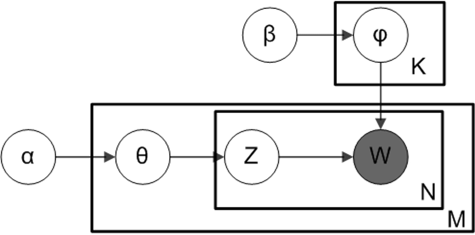
Topic models are generally represented by a plate-notation diagram as shown below source. The rectangles (also called plates in the diagram) represent loops, while the circles represent variables. The $\alpha$ and $\beta$ priors are consumed by $\Theta$ and $\Phi$ representing document-topic and topic-word distributions, respectively. W represents the sampled word, while Z is the topic assigned to it. K, M, and N are the loop stopping conditions representing the number of topics, the number of documents in the corpus, and the number of words in the topics, respectively. It can also be observed that among all variables, only W has a gray background, as it is the only known variable.

$\Theta_{d, t} = \frac{\eta_{d, t}^{-} + \alpha}{\sum_{k}^{K} \eta_{d,k}^{-} + K\alpha}$

and

$\Phi_{t, w} = \frac{\eta_{t, w}^{-} + \beta}{\sum_{v}^{V} \eta_{t,v}^{-} + V\beta}$

$P(z = t | z_-, w, d, .) = \Theta_{d, t} \times \Phi_{t, w}$

Where, w is the sampled word from d^{th} document, whose probability is computed for topic t in $\Theta_{d, t}$. The denominator normalizes the probabilities, having K as the total number of topics. $\Phi_{t, w}$ computes the probability of word w for topic t, where V is the vocabulary size. $\eta$ represents frequency e.g., $\eta_{d,t}$ means the number of times topic t appears in document d. While - is for excluding the scores of the sampled word to avoid bias in favor of the present topic.

The Vanilla implementation offers higher transparency and thus more control over the internal decisions of the method.

Contact details

M. Taimoor Khan taimoor.khan@gesis.org