
Discovering stochastic dynamical equations from ecological time series data, together with an easy to use Python package.
If you are using this software package or any code from this repo in your research, please cite us as follows:
Nabeel, A., Karichannavar, A., Palathingal, S., Jhawar, J., Brückner, D. B., Danny Raj, M., & Guttal, V., "Discovering stochastic dynamical equations from ecological time series data", arXiv preprint arXiv:2205.02645, to appear in The American Naturalist.
Arshed Nabeel, IISc Mathematics Initiative and Centre for Ecological Sciences, Indian Institute of Science, Bengaluru, Karnatata, 560012, India. Email: arshed@iisc.ac.in and arshed.nabeel@gmail.com
Danny Raj M, Dept of Applied Mechanics and Biomedical Engineering, IIT Madras, Chennai, 600036, India. Email: danny@iitm.ac.in
Vishwesha Guttal, Centre for Ecological Sciences, Indian Institute of Science, Bengaluru, Karnatata, 560012, India. Email: guttal@iisc.ac.in
The PyDaddy software package was developed by Arshed Nabeel and Ashwin Karichannavar.
The package uses two datasets from previously published papers, which are also made available as part of the package.
-
Fish dataset: Jhawar, Jitesh, et al. "Noise-induced schooling of fish." Nature Physics 16.4 (2020): 488-493. https://www.nature.com/articles/s41567-020-0787-y
-
Cell migration dataset: Brückner, David B., et al. "Stochastic nonlinear dynamics of confined cell migration in two-state systems." Nature Physics 15.6 (2019): 595-601. https://www.nature.com/articles/s41567-019-0445-4
PyDaddy is an open source package which is a key contribution of the manuscript Nabeel et al, arXiv:2205.02645. The basic scientific premise for this package is to discover the nature of stochasticity in ecological time series datasets. It is well known that the stochasticity can affect the dynamics of ecological systems in counter-intuitive ways. Without understanding the equations (typically, in the form of stochastic differential equations or SDEs, in short) that govern the dynamics of populations or ecosystems, it's challenging to determine the impact of randomness on real datasets. In this manuscript and accompanying package, we introduce a methodology for discovering equations (SDEs) that transforms time series data of state variables into stochastic differential equations. This approach merges traditional stochastic calculus with modern equation-discovery techniques. We showcase the generality of our method through various applications and discuss its limitations and potential pitfalls, offering diagnostic measures to address these challenges.
PyDaddy is a comprehensive and easy to use python package to discover data-derived stochastic differential equations from time series data. PyDaddy takes the time series of state variable
where
 |
|---|
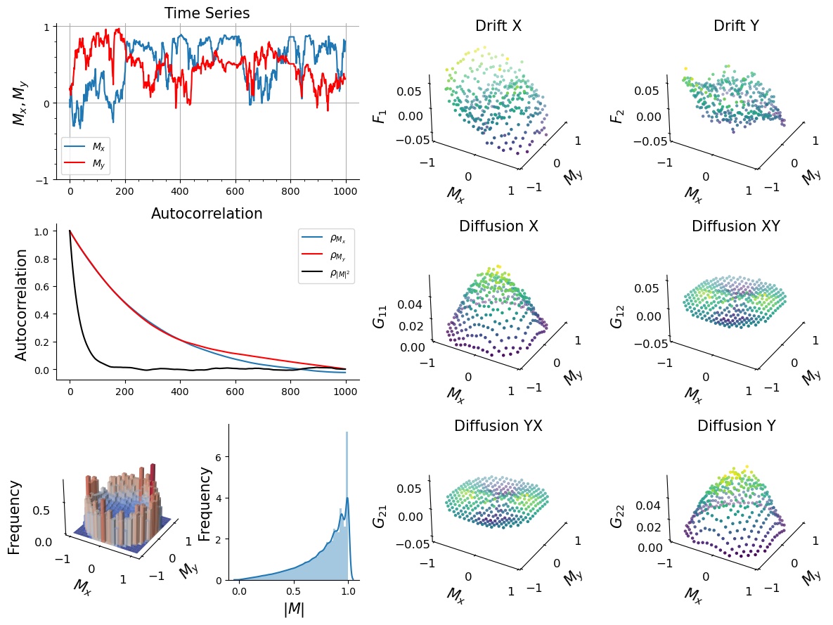
| An example summary plot generated by PyDaddy, for a vector time series dataset. |
PyDaddy also provides a range of functionality such as equation-learning for the drift and diffusion functions using sparse regresssion, a suite of diagnostic functions, etc.. For more details on how to use the package, check out the example notebooks and documentation.
The workflow of the package is summarised by the schematic given below - which is also the Fig 1 of the manuscript (https://arxiv.org/abs/2205.02645).
A detailed workflow of the package along with detailed instructions on various features are included as Supplementary Information Section S2 of the manuscript.
Detailed documentation of the PyDaddy package can be found at documentation.
 |
|---|
| Schematic illustration of PyDaddy functionality. |
We provide a number of easy to use scripts for the ease of learning and using the package, and with an aim that our manuscript is easily reproducible.
First, we emphasise that PyDaddy can be executed online on Google Colab, without having to install it on your local machine. To run PyDaddy on Colab, open a notebook on Colab. Paste the following code on a notebook cell and run it:
%pip install git+https://github.com/tee-lab/PyDaddy.git
This sets up PyDaddy in the notebook environment.
There are several example scripts / Jupyter notebooks provided, which can be used to familiarize yourself with various features and functionalities of PyDaddy. These can be executed on Colab. In the list below, we mention the path to location of each notebook as well as a link to the google colab notebook; the latter does not require installing either python or package on your system.
- Notebook 1 (notebooks/1_getting_started.ipynb): Getting started with scalar data: Introduction to the basic functionalities of PyDaddy, using a 1-dimensional dataset.
- Notebook 2 (notebooks/2_getting_started_vector.ipynb): Getting started with vector data: Introduction to the basic functionalities of PyDaddy on 2-dimensional datasets.
- Notebook 3 (notebooks/3_advanced_function_fitting.ipynb): Advanced function fitting: PyDaddy can discover analytical expressions for the drift and diffusion functions. This notebook describes how to customize the fitting procedure to obtain best results.
- Notebook 4 (notebooks/4_sdes_from_simulated_timeseries.ipynb): Recovering SDEs from synthetic time series: This notebook generates a simulated time series from a user-specified SDE, and uses PyDaddy to recover the drift and diffusion functions from the simulated time series.
- Notebook 5 (notebooks/5_exporting_data.ipynb): Exporting data: Demonstrates how to export the recovered drift and diffusion data as CSV files or Pandas data-frames.
- Notebook 6 (notebooks/6_non_poly_function_fitting.ipynb): Fitting non-polynomial functions: PyDaddy fits polynomial functions to drift and diffusion by default. This behaviour can be customized, this notebook illustrates how to do this.
- Notebook 9 (notebooks/9_higher_dimensions.ipynb): Demonstration with a 3-dimensional system An example to demonstrate that, in principle, the method of stochastic equation discovery can be extended to higher dimensions.
(See below for Notebooks 7 and 8).
There are also two notebooks that use PyDaddy to discover SDEs from real-world datasets.
-
Fish Schooling Dataset (pydaddy/data/fish_data/ectroplus.csv): The fish dataset contains the 2D polarisation vector time series of a fish school (15 fish). Two columns in the csv file represent the x- and y-components of the polarisation vector, respectively and each row corresponds to a time stamp, with consecutive rows separated by a time frame of 0.04 seconds. The full dataset is available at a previously published repository: https://zenodo.org/records/3632470. For more details about the dataset, see (Jhawar et. al., Nature Physics, 2020)[https://doi.org/10.1038/s41567-020-0787-y].
- Notebook 7 (notebooks/7_example_fish_school.ipynb): Example analysis - fish schooling: An example analysis of a fish schooling dataset from Jhawar et. al., Nature Physics, 2020 using PyDaddy.
-
Cell Migration Dataset (pydaddy/data/cell_data/trajectories_x_pattern5.txt): The confine cell migration dataset contains tracked trajectories of 149 cells, tracked for upto 300 time steps each, with one data point every 15 minutes. The data is provided as a plain text file. Each row corresponds to the time series of one cell, with each column corresponding to the cell x-position (in micrometer units). For more details about the dataset, see (Brückner et. al., Nature Physics, 2019)[https://doi.org/10.1038/s41567-019-0445-4].
- Notebook 8 (notebooks/8_example_cell_migration.ipynb): Example analysis - cell migration: An example analysis of a confined cell migration dataset (Brückner et. al., Nature Physics, 2019)[https://doi.org/10.1038/s41567-019-0445-4] using PyDaddy.
The zipped folder of codes and data is structured as follows:
- The root folder contains mostly metadata, such as readme, license etc. as well as metadata required for installation of the package.
- doc contains comprehensive documentation to the package, auto-generated by Sphinx.
- notebooks contains nine well commented/documented jupyter-notebooks/scripts which help the readers to familiarise with the usage of the package.
- pydaddy Is the main folder of the package, and contains all the main code and datasets.
- pydaddy/data folder contains three subfolders containing key real and model datasets:
- fish_data Contains the fish-schooling datasets.
- cell_data Contains the cell migration dataset (see above).
- model_data Contains simulated datasets, generated with Gillespie stochastic simulations. The models used are both scalar and vector versions of simple interaction models, as described in detail in Jhawar et. al., Nature Physics, 2020 and Jhawar & Guttal, Phil. Trans. B, 2020.
PyDaddy is available both on PyPI and Anaconda Cloud, and can be installed on any system with a Python 3 environment. If you don't have Python 3 installed on your system, we recommend using Anaconda or Miniconda. See the PyDaddy package documentation for detailed installation instructions.


To install the latest stable release version of PyDaddy, use:
pip install pydaddy
To install the latest development version of PyDaddy, use:
pip install git+https://github.com/tee-lab/PyDaddy.git


To install using conda, Anaconda or Miniconda need to be installed first. Once this is done, use the following command.
conda install -c tee-lab pydaddy
For more information about PyDaddy, check out the package documentation.
If you are using this package in your research, please cite the associated paper as follows:
Nabeel, A., Karichannavar, A., Palathingal, S., Jhawar, J., Brückner, D. B., Danny Raj, M., & Guttal, V., "Discovering stochastic dynamical equations from ecological time series data", arXiv preprint arXiv:2205.02645, to appear in The American Naturalist.
This study was partially funded by Science and Engineering Research Board, Department of Science and Technology, Government of India to Vishwesha Guttal.
PyDaddy is distributed under the GNU General Public License v3.0.