https://www.zcyphygeodesy.com/en/h-nd-153.html
From a single type of observations selected from the residual gravity disturbance (mGal), height anomaly (m), gravity anomaly (mGal), disturbing gravity gradient (E, radial) or vertical deflection (″), and a kind of spherical radial basis functions (SRBFs) selected from the point mass Kernel function, Poisson kernel function, m-order radial multipole kernel or m-order wavelet kernel function, estimate the residual gravity disturbance, height anomaly, gravity anomaly, disturbing gravity gradient or vertical deflection on or outside the geoid.
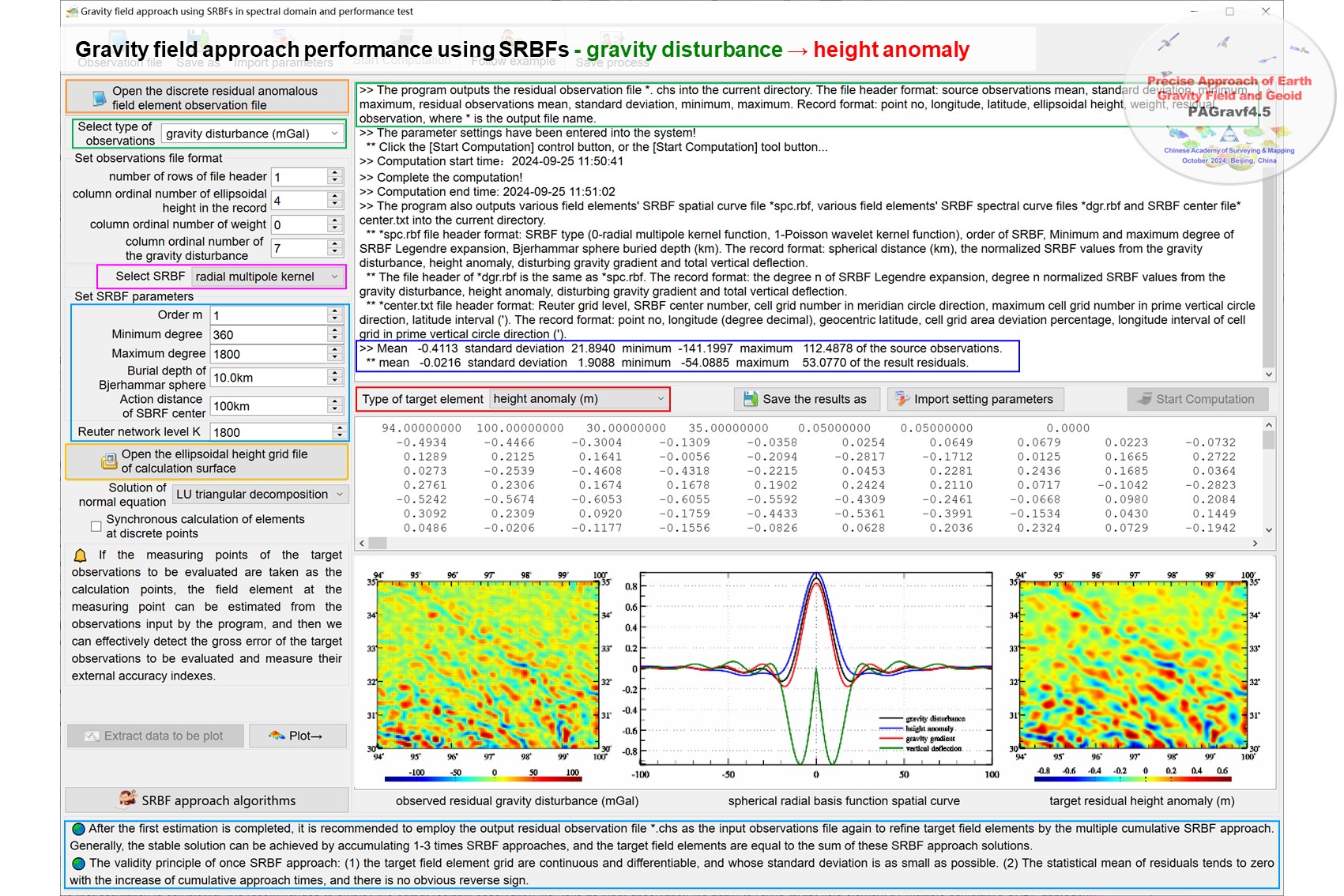
From a single type of residual anomalous field observations and a kind of spherical radial basis functions (SRBFs), estimate the residual anomalous field element grid on or outside the geoid.
Selecting different type of observations and constructing different figure of SRBF, we can calculate different type of target field elements, and then fully verify and analyze the spatial and spectral properties of gravity field approach algorithms using SRBFs.
Setting the observation weight of the target field element to be evaluated to zero, or directly taking the observed point of the target field element to be evaluated as the calculation point, we can effectively detect the gross error of the target observations and measure their external accuracy indexes.
The program itself can be employed for analytical continuation, griding, type conversion and all-element modelling on gravity field from various single type of observed field elements.

GravityfieldapproachSRBFtest.f90
Input parameter: observationfl - The discrete residual anomalous field element observation file name.
 ▪ The file header occupies one line and the record format: ID (point no / point name), longitude (decimal degrees), latitude (decimal degrees), ellipsoidal height (m), …, observation, …, weight,…
Input parameter: surfhgtgrdfl - The ellipsoidal height grid file name of the calculation surface.
Input parameter: checkpointfl - The checkpoint file name.
 ▪ The checkpoint file can be employed to detect effectively the gross error of the target observations to be evaluated and measure their external accuracy indexes.
 ▪ The file header occupies one row and the record format: ID (point no / point name), longitude (decimal degrees), latitude (decimal degrees), ellipsoidal height (m), …
Input parameters: para(1:7) - the minimum and maximum degree of SRBF Legendre expansion, the order number m, the spherical radial basis functions (=0 radial multipole kernel function, =1 Poisson wavelet kernel function), Reuter network level K, action distance (km) of SRBF center and Bjerhammar sphere burial depth (km).
Input parameters: para(8:9) - the types of the observation and unknown target field elements.
Input parameters: para(10:11) - the column ordinal number of the observation field element in the observation file record. When para(8) = 2, para(10:11) are the column ordinal numbers of observation vertical deflection (SW).
Input parameter: para(12) - the column ordinal number of the observation weight.
 ▪ When the column ordinal number of the weight attribute is less than 1, exceeds the column number of the record, or the weight is less than zero, the program makes the weight equal to 1.
 ▪ When the weight in the file record is equal to zero, the observation will not participate in the estimation of the SRBF coefficient, and the program can be employed to measure the external accuracy index of the observations.
Input parameters: para(13) - method of the solution of normal equation. =1 LU triangular decomposition method, =2 Cholesky decomposition, =3 least square QR decomposition, =4 Minimum norm singular value decomposition and =5 ridge dstimation.
SRBFestimation(observationfl,surfhgtgrdfl,checkpointfl,para)
Input parameter: observationfl - The discrete residual anomalous field element observation file name.
Input parameter: surfhgtgrdfl - The ellipsoidal height grid file name of the calculation surface.
Input parameter: checkpointfl - The checkpoint file name.
Output the approached target field element grid file SRBFestimate.dat  with the same grid specifications as the ellipsoidal height grid file of the calculation surface.
The module also outputs the residual observation file residuals.txt and checkpoint target field element file checkreslt.txt.
 ▪ The header format of the file residuals.txt : source observations mean, standard deviation, minimum, maximum, residual observations mean, standard deviation, minimum, maximum. The record format: ID, longitude, latitude, ellipsoidal height, weight, source observation, residual observation.
 ▪ The record format of the file checkreslt.txt: Behind the check point file record, appends a column of residual observation element approached.
The module also outputs the SRBF spatial curve file SRBFspc.txt, spectral curve file SRBFdgr.txt of 5 kinds of field elements and SRBF center file SRBFcenter.txt into the current directory.
SRBFspc.txt file header format: SRBF type (0-radial multipole kernel function, 1-Poisson wavelet kernel function), order of SRBF, Minimum and maximum degree of SRBF Legendre expansion, Bjerhammar sphere buried depth (km). The record format: spherical distance (km), the normalized SRBF values from the gravity disturbance, height anomaly, disturbing gravity gradient and total vertical deflection.
The file header of SRBFdgr.txt is the same as SRBFspc.txt. The record format: the degree n of SRBF Legendre expansion, degree n normalized SRBF values from the gravity disturbance, height anomaly, disturbing gravity gradient and total vertical deflection.
SRBFcenter.txt file header format: Reuter grid level, SRBF center number, cell-grid number in meridian circle direction, maximum cell-grid number in prime vertical circle direction, latitude interval ('). The record format: point no, longitude (degree decimal), geocentric latitude, cell-grid area deviation percentage, longitude interval of cell-grid in prime vertical circle direction (').
ReuterGrid(rhd,lvl,Kt,blat,nn,mm,nln,sr,dl,nrd,lon)
Input parameters: rhd(4) - minimum and maximum longitude, minimum and maximum geocentric latitude of the Reuter network.
Input parameters: lvl, nn, mm - the Reuter network level, maximum number of Reuter centers in the meridian direction and that in the parallel direction.
Return parameter: Blat - the geocentric latitude (degree decimal) of Reuter centers in the first parallel direction.
Return parameters: Kt - the number of Reuter centers, equal to the number of unknowns to be estimated.
Return parameters: nln(nn) - the number of the Reuter centers in the parallel direction.
Return parameters: sr(nn) - the percentage of the difference between the area of the Reuter cell-grid in the parallel direction and the area of the equatorial cell-grid.
Return parameters: dl(nn) - the longitude interval (degree decimal) of the Reuter centers in the parallel direction.
Return parameters: nrd(nn,mm) - ordinal number value of the Reuter centers.
Return parameters: lon(nn,mm) - longitude value of the Reuter centers.
Edgnode(enode,rlatlon,lvl,edgn,lon,blat,nln,gpnt,nn,mm)
The module calculates the number of observation points in the Reuter cell-grid and the number gpnt of Reuter centers corrected.
Return parameter: edgn - the number of Reuter centers around the edge of the Reuter grid.
Return parameters: enode(edgn) - the ordinal number value of Reuter centers in the edge of the Reuter grid.
Return parameter: rlatlon(edgn,2) - the geocentric latitude and longitude (degree decimal) of Reuter centers in the edge of the Reuter grid.
SRBF5all(RBF,order,krbf,mpn,mdp,minN,maxN,NF,nta)
Return parameters: RBF(NF+1,5) - The SRBF curves of 5 kinds of field elements, which are calculated by the action distance of SRBF center and Reuter grid level.
 ▪ Where RBF(NF+1,knd): knd=1 gravity disturbance (mGal), =2 height anomaly (m), =3 gravity anomaly (mGal), =4 disturbing gravity gradient (E, radial) or =5 vertical deflection (″).
Input parameters: nta - the bandwidth parameter and nta = (r0-dpth)/r0, here dpth is the Bjerhammar sphere burial depth and r0 is the average geocentric distance of observation points.
Input parameters: krbf,order - krbf=0 radial multipole kernel function, =1 Poisson wavelet kernel function and order is the order number of SRBF.
Input parameters: mpn(maxN-minN+1, NF+1), mdp(maxN-minN+1, NF+1) - all minN to maxN degree Legendre functions and their first derivatives.
RtGridij(rln,ki,kj,blat,lvl,nn,mm,nln,dl,lon)
Input parameters: rln(3) - the spherical coordinates of the calculation point。
Return parameters: ki,kj - the position of the calculation point rln(3) in the Reuter grid, It is represented by the element of the 2-D ordinal number array of the Reuter grid and ki>0, kj>0.
Equsolve(BB,xx,nn,BL,knd,bf)
The mkl_lapack95_ilp64.lib library is called to solve the large equations BB.xx = BL. bf(8) is the property of the solution.
Input parameter: knd - method of the solution of normal equation and knd =1 LU triangular decomposition method, =2 Cholesky decomposition, =3 least square QR decomposition, =4 Minimum norm singular value decomposition.
normdjn(GRS,djn); GNormalfd(BLH,NFD,GRS)
Return parameters: NFD(5) - the normal geopotential (m2/s2), normal gravity (mGal), normal gravity gradient (E), normal gravity line direction (', expressed by its north declination relative to the center of the Earth center of mass) or normal gravity gradient direction (', expressed by its north declination relative to the Earth center of mass).
LegPn_dt1(pn,dp1,n,t) ! t=cos ψ
BLH_RLAT(GRS, BLH, RLAT); RLAT_BLH(GRS, RLAT, BLH)
LegPn02(mpn,mdp,mp2,minN,maxN,NF,dr); PickRecord(line, kln, rec, nn)
RBFvalue(RBF(:,1),NF,dr,dln(2),tmp); drln(rln,rlnk,dln); Stat1d(dt,nn,rst)
Fortran90, 132 Columns fixed format. Fortran compiler. mkl_lapack95_ilp64.lib link library required.
[Algorithmic formula] PAGravf4.5 User Reference https://www.zcyphygeodesy.com/en/
7.10 Theory and algorithm of gravity field approach using spherical radial basis functions
The zip compression package iincludes the test project in visual studio 2017 - intel fortran integrated environment, DOS executable test file and all input and output data.


