LogFileAnalysis1

Log file analysis example: Nadia with IHMC walking controller

In this example we will use the log file of the humanoid robot Nadia using the IHMC walking controller to show how to use the log file analysis tool.

Download the log file

The log file is available at Google Drive. Download the file and unzip it. You should have a folder named 20231208_NadiaLogExampleWithFall that looks like this:

20231208_NadiaLogExampleWithFall
├── handshake.yaml
├── model.sdf
├── NadiaPoleNorth_Timestamps.dat
├── NadiaPoleNorth_Video.mov
├── NadiaTripodSouth_Timestamps.dat
├── NadiaTripodSouth_Video.mov
├── resources.zip
├── robotData.bsz
├── robotData.dat
├── robotData.log
├── ValkyrieTripodNorth_Timestamps.dat
└── ValkyrieTripodNorth_Video.mov

Load the log file

Assuming you have the scs2 package installed ( see README.md), start SCS2 Session Visualizer.

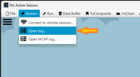
A new window will open:

Click on the Open Log... button and select the robotData.log file in the 20231208_NadiaLogExampleWithFall folder.

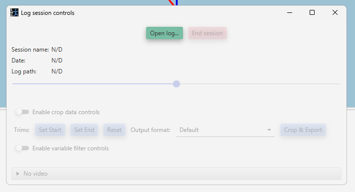
After a short while, the window will look like this:

Here you see the controls updated as follows:

1. The name of the log session, the date and time of the log session, and the path to the log file.
2. The slider allows to scrub through the log file. However, note that when scrubbing, the log file is not actually loaded into the memory. This means that the data is not available for analysis.
3. Controls for cropping the log file. Log files are typically large, so cropping can be useful when you want to share a log file with someone else. This log was already cropped, so we won't use this feature here.
4. The bottom part of the window shows any video files that are associated with the log file. You can double-click on a thumbnail to open the video file in a separate window.

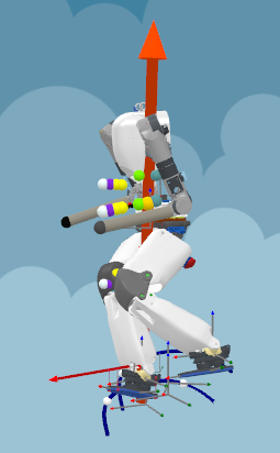
In the main window, you should see the robot by zooming out (use the mouse wheel):

Use the mouse to rotate the view:

1. Left click and drag to rotate the camera about its focal point (the focal point is initialized at (0,0,0)).
2. Right click and drag to rotate the camera about itself.
3. Use WASD to move the camera in the horizontal plane and QZ to move the camera up and down.
4. Hold shift and left click on a graphic (e.g. the robot) to move the focal point to that graphic.
5. Right click on a graphic to open a context menu. For example, you can select Track to track the graphic.

Let's move the camera to the robot pelvis, and track it:

Log the log file in memory

Now we want to load the log file into memory. To do this, click on the gear button in the main window:

After clicking on the gear button, you should see the scrubbing slider move and Nadia move as well. Let's wait until it's done.

Playing back the log file

When loading the log file into memory, as we just did, it will read the log as fast as possible. To see robot move at the real-time speed, hit the play button ( next to the gear). Now you should see Nadia moving at the real-time speed.

Note: You can change the playback speed through the menu Run > Playback real-time rate, it is initialized to 1.0.

Note: While playing back, the videos from the logging cameras are also played back. Double click on a video thumbnail to open it in a separate window.

Overhead view

Let's open the overhead view. Go to YoGraphics > Overhead Plotter. A new pane should open:

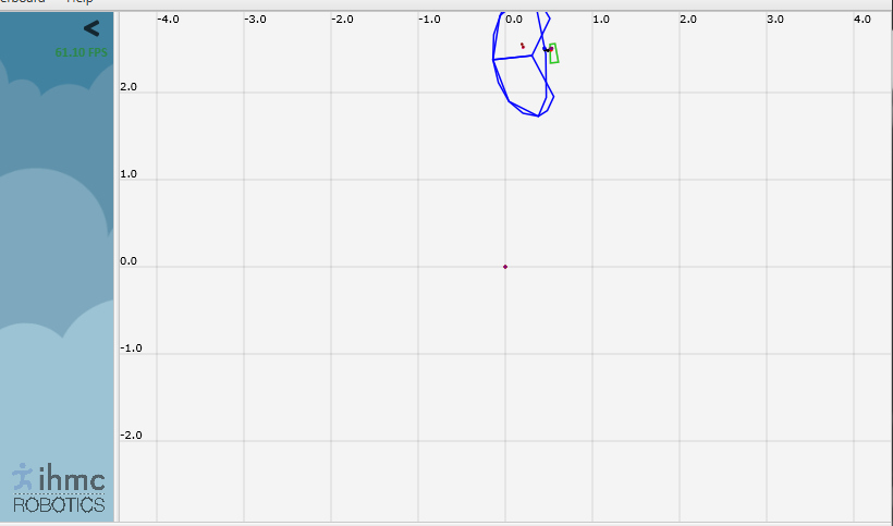
The overhead view is a 2D topdown view of the robot (well without the robot actually). We use it to plot data that is critical to the robot balance such as the robot's center of mass (CoM) and the support polygon.

Camera controls:

1. Left click and drag to pan the camera.
2. Mouse wheel to zoom in and out.
3. To track a coordinate, go to the menu YoGraphics > Plotter Options... and select the variables you want to track.

Let's add the CoM to the overhead view (we will pretend that it is not already there). Go to YoGraphics > YoGraphic properties.... A new window should open:

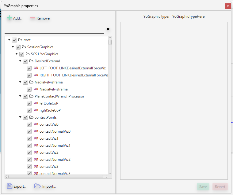
Click on the Add... button. A new window should open:

Let's select the point in the 2D graphics section (should already be open), at the bottom, let's name our new graphic like My own CoM, finally click on the Create button.

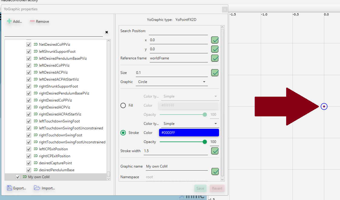
The new graphic should appear in the list of YoGraphics, it also shows up in the overhead view at the coordinate (0, 0). Hovering the mouse over the new graphic will display its name, it's a convenient way to identify a graphic in the overhead view and understand what it represents.

Let's configure the graphic, so it tracks Nadia CoM, the editor is already up on the right side of the YoGraphic properties window. Let's do it:

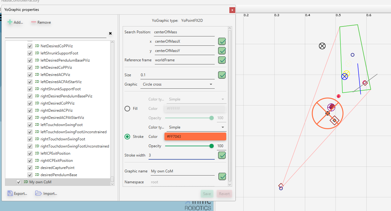
If you play the log file, you should see the CoM moving in the overhead view.

You can use the same procedure to add other types of graphics in the overhead plotter and as well as in the main viewport.

Let's plot data!!

Alright, now let's open some charts and plot data! In the top left corner of the main window, click on the hamburger button: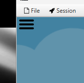

A new pane should open:

There you can search for variables to plot. Let's search for the robot's CoM. Type centerOfMass in the search bar. You should see a list of variables that contain the string centerOfMass:

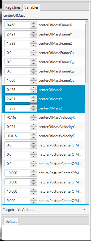
Now let's first create 3 charts. Click on the little blue arrow pointing downward:

A mini chart table should appear:

Let's make 3 charts horizontal by clicking on the table's cell located on the first row and third column. Three empty charts should appear:

Now let's select the 3 components of the robot's CoM and drag them into the first chart. A little popup should show up in which you can select either Single or Horizontal. Let's select horizontal. You should end up with this:

Alright! You know the basics of plotting data. You can drag and drop additional variables into the charts, you can also drag and drop variables from one chart to compare them over time.

Notes;

• left click and drag on a chart to scrub through the loaded part of the log file.
• the mouse wheel also scrubs through the loaded part of the log file.
• use the magnifier button to zoom in and out on all the charts of a window.
• right click and drag on a chart to pan it.
• use the menu option: YoChart > New chart window to create a new chart window.

Why Nadia fell?

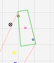
Let's use the tools to identify why Nadia fell. In the overhead view, you can see that Nadia fell on her right side at the beginning of the last step.

We can see that the center of pressure was all the way in the corner of the support polygon, which is a good sign in the sense that the controller was attempting to recover balance.

Let's back up in time and look at the transfer leading to the fall, right there:

We can see that in each foot, the center of pressure isn't tracking at all:

I highlighted the desired and measured center of pressures in the right foot. Similar behavior is observed in the left foot.

Let's plot the desired and measured center of pressure for both feet:

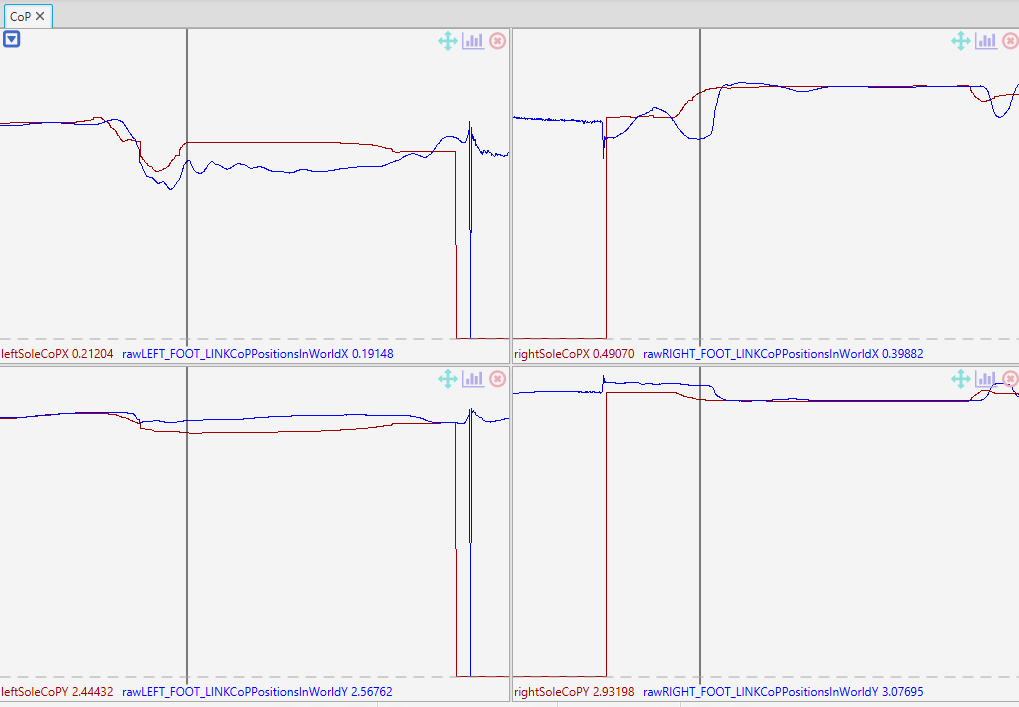
We can see the tracking for the right foot is quite bad right after touchdown and then recovers. This is typical problem we deal with with our hydraulic actuators in the ankle, they don't provide sufficient force control while barely loaded. Let's confirm that by looking at the joint torque tracking:

As for the left foot, the CoP was tracking well early in the transfer, but degraded during transfer. Looking at the rear ankle joint configuration, we can see that the ankle hit its joint limit:

While q_min and q_max are not exactly equal to the joint limits, because they're assumed to be constant which is not correct for large angle combinations for both pitch and roll, we can see that the force tracking remains great while CoP tracking isn't. This can only mean that forces are being distributed in the ankle joint, which is a sign that the ankle is hitting its joint limit.

Conclusion

In this example, we saw how to load a log file, play it back, add graphics to the overhead view, and plot data. We also saw how to use the tools to identify why a robot fell. Go ahead and play with the tools.