-
Notifications
You must be signed in to change notification settings - Fork 25
DQN Maze Solver
In my previous post I showed how to build a maze-solving Q-learner using a table-based Q-learning method. In this post, I show how to solve the same maze using DQN (Deep Q-Learning). The code for this example program is found here.
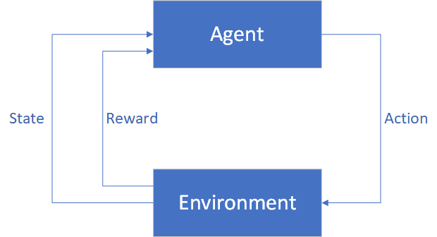
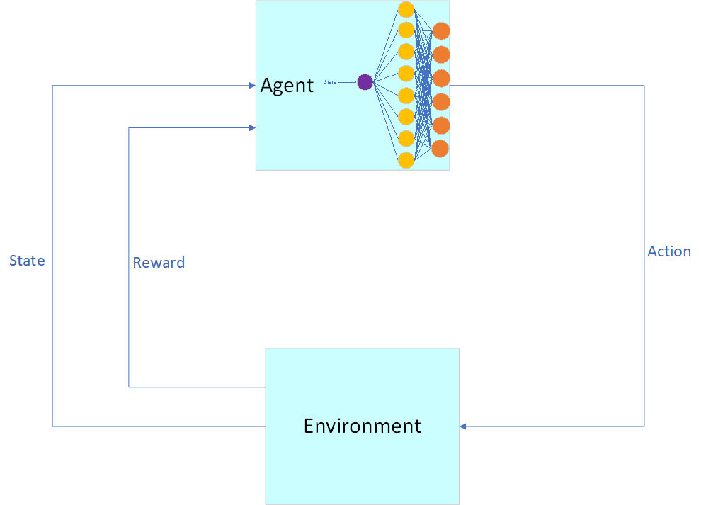
In a reinforcement learning problem, an Agent interacts with an Environment by evaluating its State, taking Actions, and receiving Rewards. The goal is to learn which Actions provide the most Reward over the course of time.
 # The Maze Problem
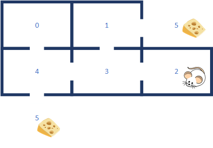
As in the previous post, we’re going to attempt to solve the maze problem. A mouse gets dropped randomly into 1 of 6 places on the maze and must learn to find the cheese (reward).

Just as in the previous post, we define the maze in the program as follows:
/*
Q-Learning unit test. Learn the best path out of a simple maze.
5 == Outside the maze
________________________________________________
|                       |                       |
|                       |                       |
|           0           |          1             / 5
|                       |                       |
|____________/  ________|__/  __________________|_______________________
|                       |                       |                       |
|                       |                        /                      |
|           4           |          3            |           2           |
|                        /                      |                       |
|__/  __________________|_______________________|_______________________|
    5
The paths out of the maze:0->4->5
0->4->3->1->5
1->5
1->3->4->5
2->3->1->5
2->3->4->5
3->1->5
3->4->5
4->5
4->3->1->5
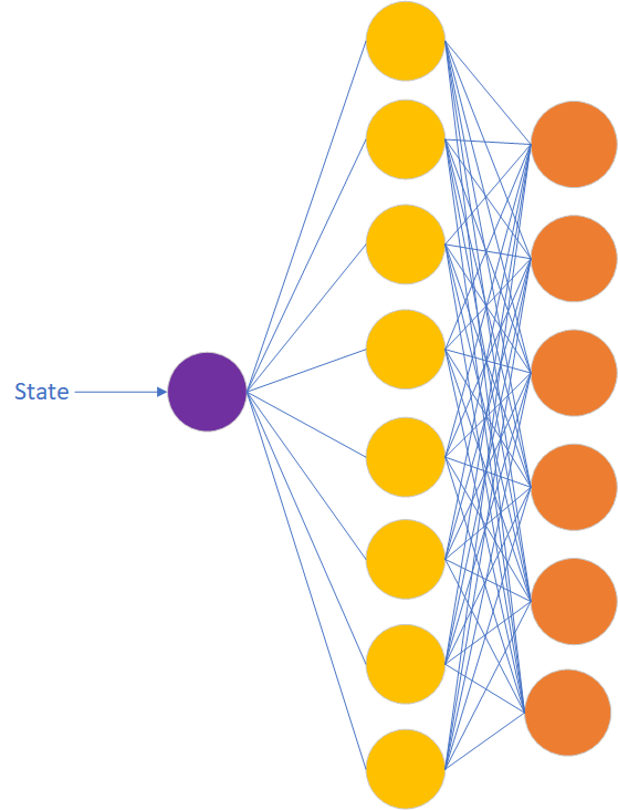
For this problem we will get rid of the Q-table from the previous post and replace it with a neural network. We will need 1 input neuron (State) and 6 output neurons (Actions). I’ve chosen to implement 1 hidden layer with 2 more neurons than output neurons (it just felt right). Each output neuron represents the action to take from the state. There is 1 neuron in the input layer, which represents the current state of our mouse. Using Q-format, I scale the input by taking the current state and dividing by the maximum possible state (i.e. 5, 6 states in total numbered 0–5). To do this, the DQN neural network queries the Environment and expects it to initialize the pointer to an array of inputs to the neural network for a given numeric representation of state.
template<typename StateType,
         typename ActionType,
         typename ValueType,
         size_t NumberOfStates,
         size_t NumberOfActions,
         typename RewardPolicyType,
         template<typename> class QLearningPolicy = tinymind::DefaultLearningPolicy
         >
struct DQNMazeEnvironment : public tinymind::QLearningEnvironment<state_t, action_t, ValueType, NumberOfStates, NumberOfActions, DQNMazeEnvironmentRandomNumberGeneratorPolicy>
{
...
static void getInputValues(const StateType state, ValueType *pInputs)
{
    static const ValueType MAX_STATE = ValueType((NumberOfStates - 1),0);
    ValueType input = (ValueType(state, 0) / MAX_STATE);
    *pInputs = input;
}
Another way to accomplish this would have been to have 6 input neurons. But, this method works just fine since we have 16 bits of resolution and only 6 states.
The neural network code used is also from cppnnml. To get some insight into how these neural networks work see my articles here and here. The neural network is trained to predict the Q-value for every action taken from the given state. After the neural network is trained, we then choose the action which contains the highest Q-value (i.e. output neuron 0 == action 0, output neuron 1 == action 1, etc.).

Figure 1: Neural Network Architecture For DQN Example Maze Solver

Figure 2: The Agent Uses A Neural Network To Get/Set Q Values
The DQN is defined within dqn_mazelearner.h.
Change directories to the example code at cppnnml/examples/dqn_maze. We create a directory to hold the built executable program and then compile the example. We need to compile the neural network LUT code as we all as define the type(s) of LUTs to compile. In this case, we only need the tanh activation function for a signed Q-format type of Q16.16. See this article for a detailed explanation of how neural networks within cppnnml work.
mkdir -p ~/dqn_maze
g++ -O3 -o ~/dqn_maze/dqn_maze dqn_maze.cpp dqn_mazelearner.cpp ../../cpp/lookupTables.cpp -I../../cpp -I../../apps/include/ -DTINYMIND_USE_TANH_16_16
This builds the maze leaner example program and places the executable file at ~/dqn_maze. We can now cd into the directory where the executable file was generated and run the example program.
cd ~/dqn_maze
./dqn_maze
When the program finishes running, you’ll see the last of the output messages, something like this:
take action 5
*** starting in state 4 ***
take action 5
*** starting in state 5 ***
take action 1
take action 5
*** starting in state 2 ***
take action 3
take action 1
take action 5
*** starting in state 0 ***
take action 4
take action 5
*** starting in state 1 ***
take action 5
*** starting in state 1 ***
take action 5
*** starting in state 3 ***
take action 1
take action 5
*** starting in state 5 ***
take action 1
take action 5
*** starting in state 4 ***
take action 5
Your messages may be slightly different since we’re starting our mouse in a random room on every iteration. During example program execution, we save all mouse activity to files (dqn_maze_training.txt and dqn_maze_test.txt). Within the training file, the mouse takes random actions for the first 400 episodes and then the randomness is decreased from 100% random to 0% random for another 100 episodes. To see the first few training iterations you can do this:
head dqn_maze_training.txt
You should see something like this:
1,3,4,3,1,5,
1,3,1,5,
1,3,4,3,1,5,
5,4,5,
1,5,
2,3,1,5,
3,2,3,4,0,4,3,1,5,
4,0,4,5,
4,0,4,0,4,0,4,5,
4,0,4,5,
Again, your messages will look slightly different. The first number is the start state and every comma-separated value after that is the random movement of the mouse from room to room. Example: In the first line above we started in room 1, then moved to 3, then 4, then 1, then to 5. Since 5 is our goal state, we stopped. The reason this looks so erratic is for the first 400 iterations of training we make a random decision from our possible actions. Once we get to state 5, we get our reward and stop.
I have included a Python script to plot the training and test data. If we plot the training data for start state == 2 (i.e. the mouse is dropped into room 2 at the beginning):

Each line on the graph represents an episode where we’ve randomly placed the mouse into room 2 at the start of the episode. You can see that in the worst case run, we took 18 random moves to find the goal state (state 5). This is because at each step, we’re simply generating a random number to choose from the available actions (i.e. which room should be move to next). If we use the script to plot the testing data for start state == 2:

You can see that after we’ve completed training, the Q-learner has learned an optimal path: 2->3->1->5.
The reason we’d use a DQN rather than a table-based Q-learner would be when the number of states or complexity of the state space would make the Q-table unreasonably large. For this maze problem, this is not true. I chose this problem to show a direct comparison between table-based Q-learning and DQN, not necessarily to save any space. In fact, the DQN implementation takes up more code and data space than the table-based method. In a more complex state-space, we’d be able to realize the gains from DQN vs. table-based.
In any case, we want to measure how much code and data it takes to implement our maze-solving DQN:
g++ -c dqn_mazelearner.cpp -O3 -I../../cpp -I../../apps/include/ -DTINYMIND_USE_TANH_16_16 && mv dqn_mazelearner.o ~/dqn_maze/.

cd ~/dqn_maze/
size dqn_mazelearner.o
The output you should see is:
text data bss dec hex filename
12255 8 3652 15915 3e2b dqn_mazelearner.o
We can see that the entire DQN fits within 16KB. Pretty small as DQN goes.
As of today, there are 2 types of Q-Learning supported within cppnnml: Table-based Q-learning, and DQN. Example programs as well as unit tests exist within the repository to demonstrate their uses. DQN trades out the Q-table for a neural network to learn the relationship between states, actions, and Q-values. One would want to use DQN when the state space is large and the memory consumed by the Q-table would be prohibitively large. By using DQN, we’re trading memory for CPU cycles. The CPU overhead for DQN will be far larger than a Q-table. But, DQN allows us to do Q-learning while keeping our memory footprint manageable for complex environments.