-
Notifications
You must be signed in to change notification settings - Fork 0
MoMA tutorial preprocessing
The preprocessing performs the following steps on the full frame images in the OME-TIFF stack that was captured with MicroManager:
- It registers the frames from each position to compensate image drift/shifting between frames.
- It normalizes image intensity of the phase contrast (PhC) images to improve predictions of the U-Net model.
- It detects the location the GLs in the image.
- It splits the full frame TIFF stack into smaller TIFF stacks containing one growth lane each (GL). These stacks are referred to as GL ROIs in the following sections (ROI: region of interest).
To preprocess your data you have to perform the following steps:
- Setup the path to the preprocessing module in your .bashrc.
- Create a template image to detect GLs.
- Create a template configuration file for your template image. Template image and configuration are used to locate the GL ROIs in the full frame image.
- Configure the preprocessing bash script for your dataset.
- Run the bash script to preprocess your data.
We will go through these steps in the following sections.
The template image and configuration are used to locate the GL ROIs inside the full frame image. We start by creating a template image ...
-
Open a terminal and start MicroManager:
$ mm_1.4
Important: To use use the command mm_1.4 you will need to load the ImTools module:
$ ml ImTools
-
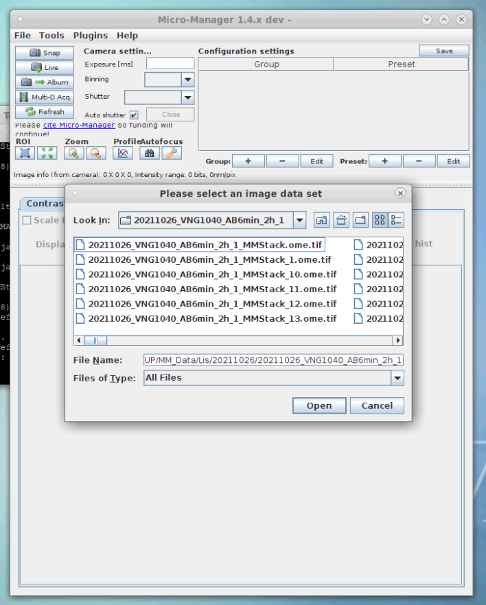
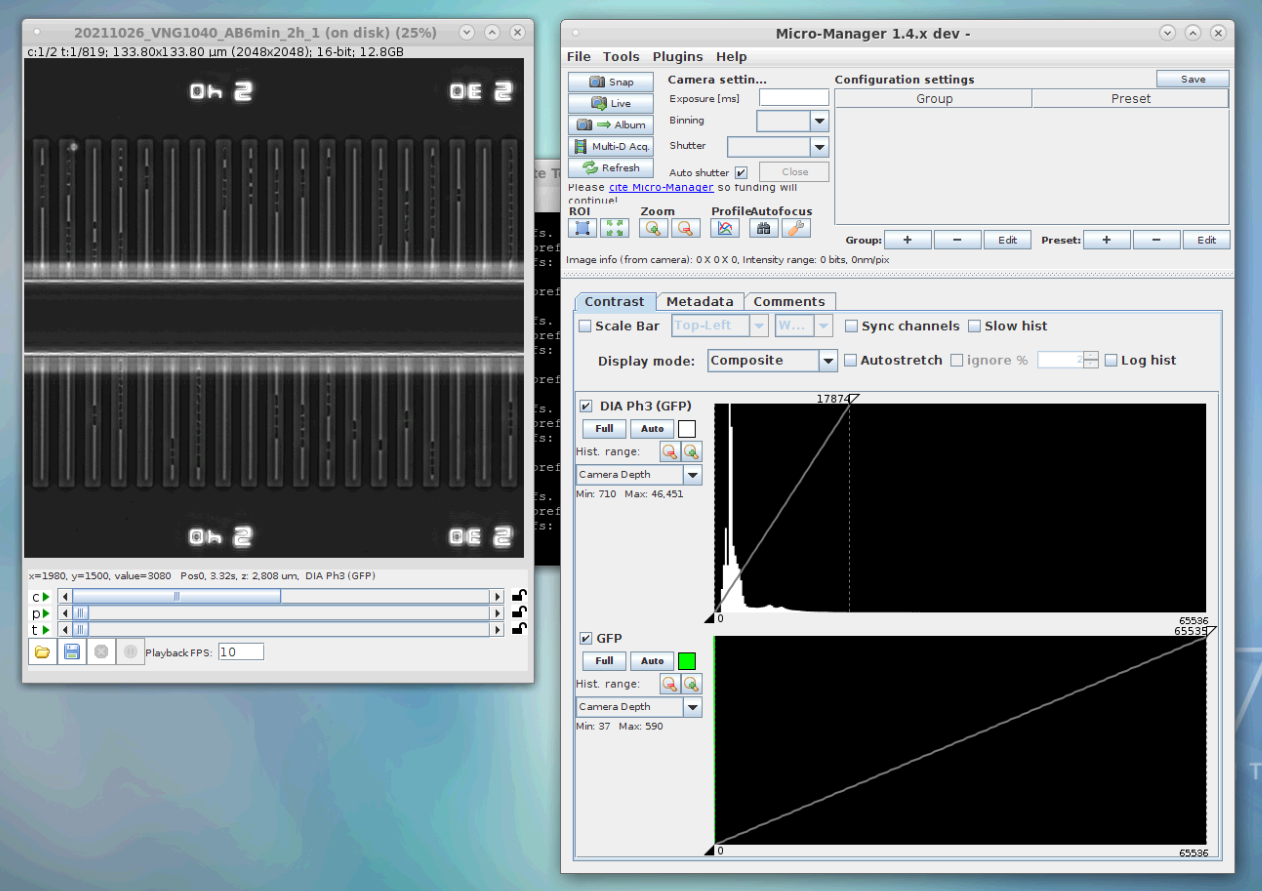
Open the OME-TIFF stack in MicroManager as virtual stack (click on the screenshots to enlarge):
Step 1: Select to open image as virtual stack. Step 2: Select image folder and open dataset. Step 3: View with opened image stack. Use the slider of in the phase contrast histogram (top) to adjust image saturation for better channel visibility. 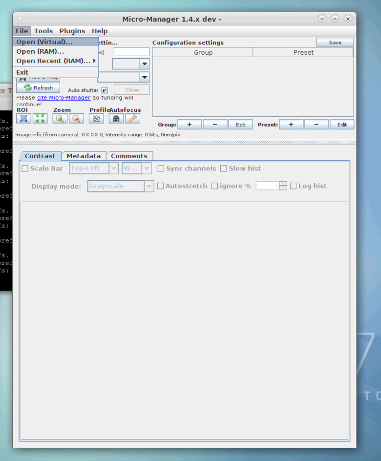
-
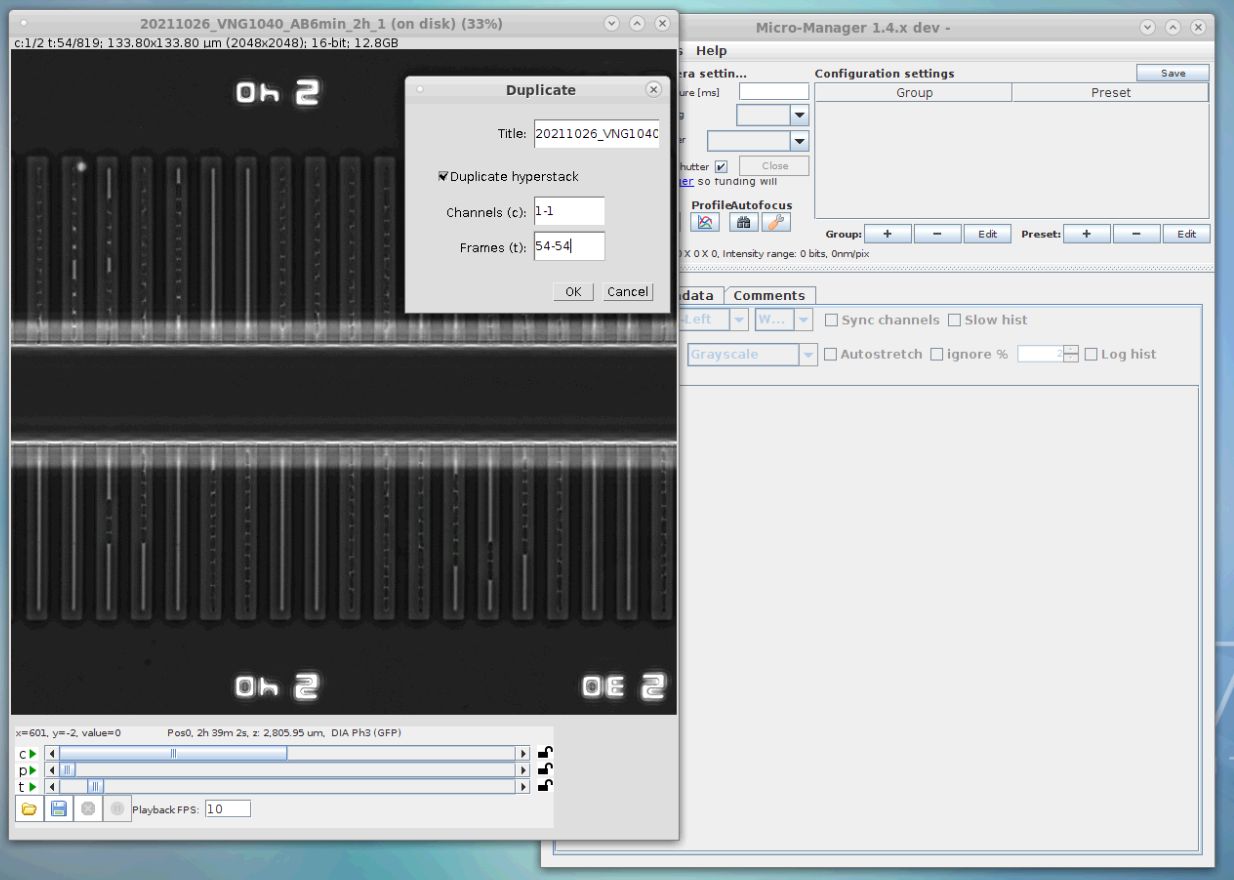
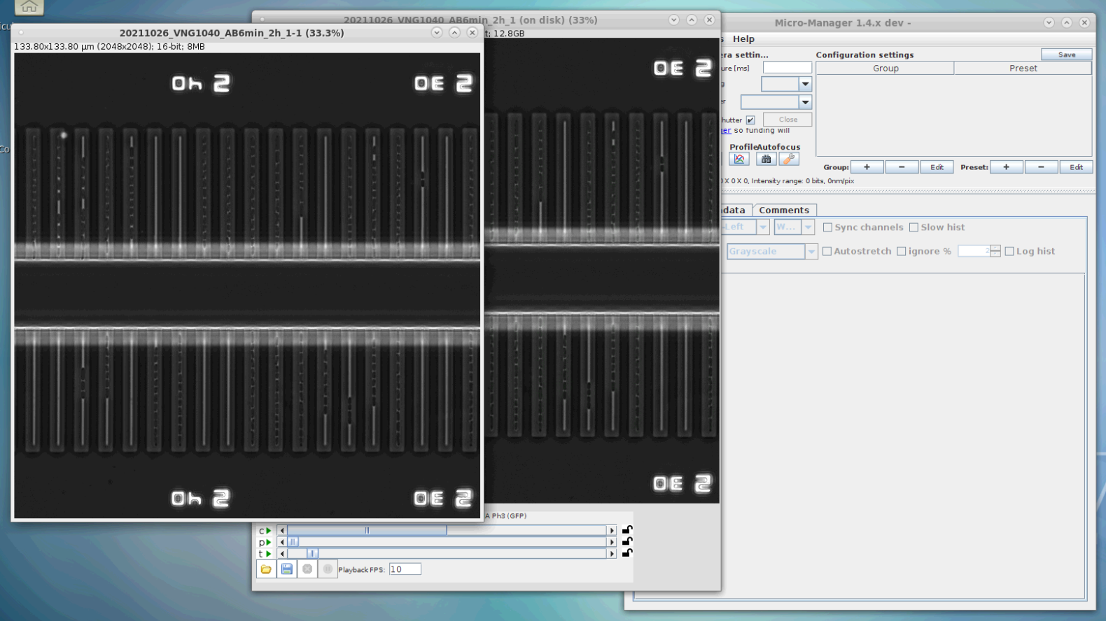
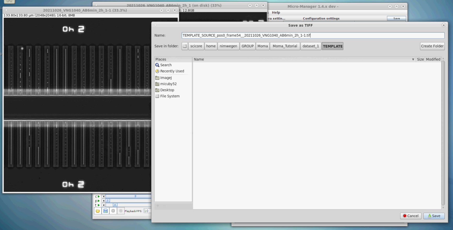
Use the sliders p and t under the image to select a position and time steps, which contains 3 adjacent, suitable GLs. We will use a crop of this region to create the template image. A suitable frame is one, which has good focus and similar appearance to the other positions and frames in the dataset. Ideally, the GLs in the template image crop should be empty, but template matching also works well with filled GLs (or a mix of filled/non-filled GLs). After you identified a suitable position and frame, duplicate it to a new image (Ctrl+Shift+D) and save it (Ctrl+S).
Step 1: Zoom into image for better using either '+' key or the magnifying glass of the ImageJ. Step 2: Open the duplicate dialog (Ctrl+Shift+D) and enter channel 1 (the PhC channel) and the frame of interest (in this case 54) Step 3: Save the duplicated image to the template folder. 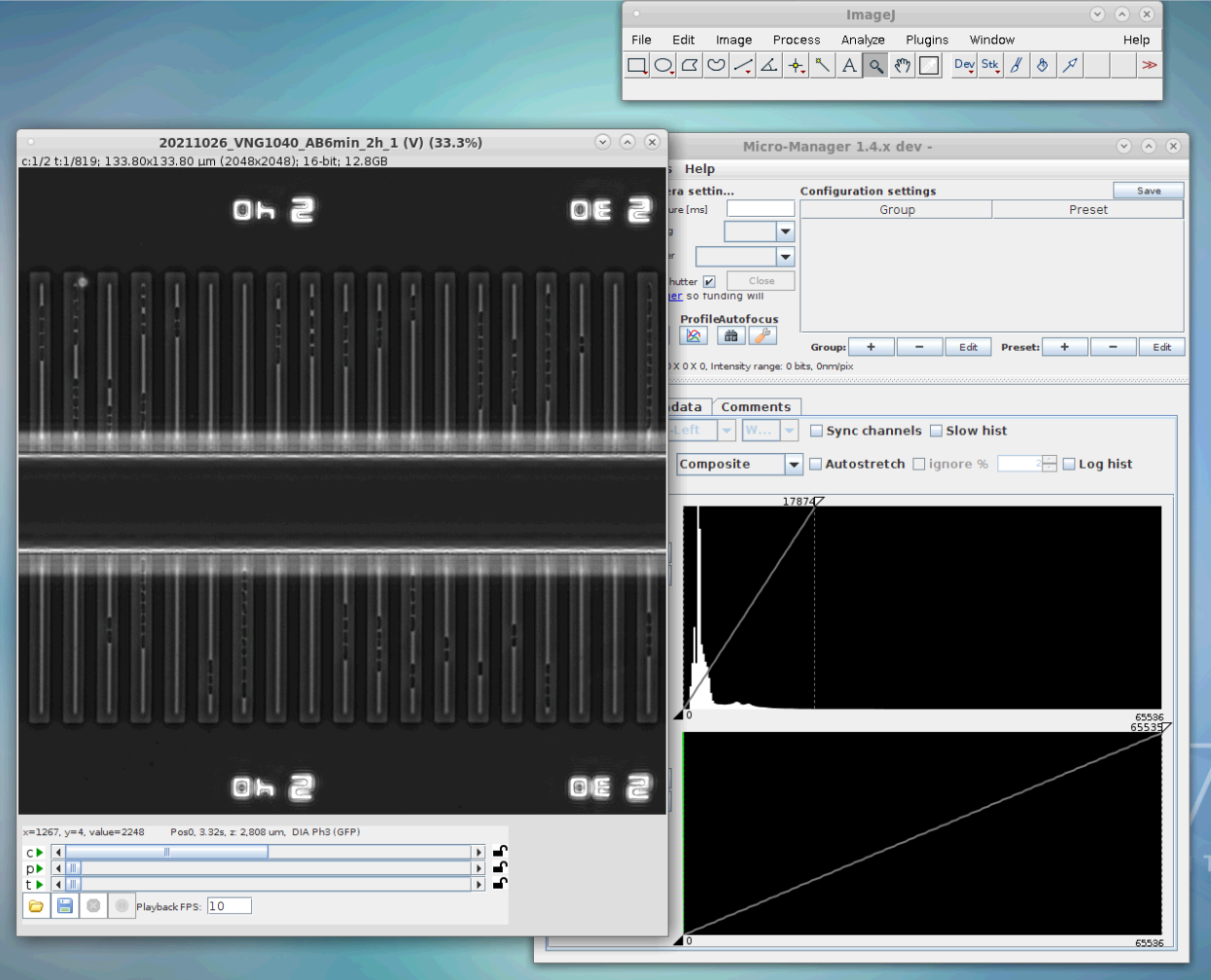
-
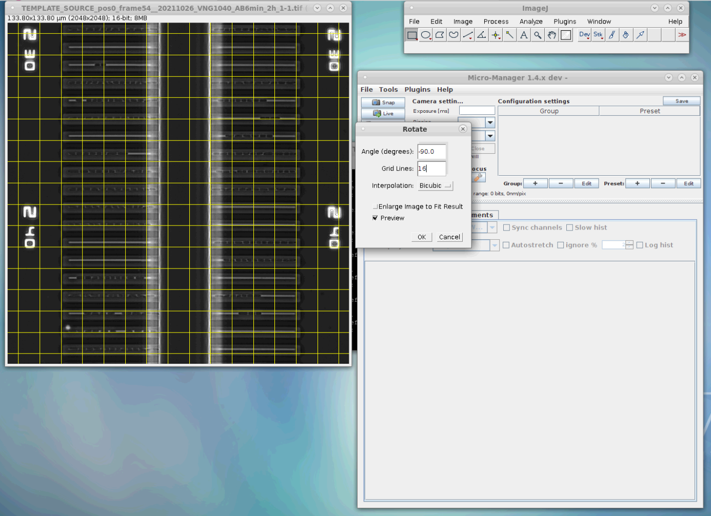
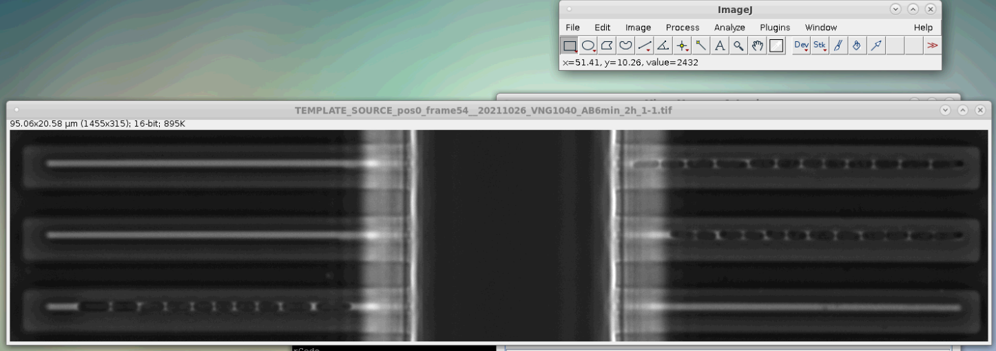
Rotate the duplicated frame (referred to from here on as template source) in counter clockwise direction (i.e. negative angle) and create a crop from the image, which will be used as template image.
Important:
Note down the rotation angle of the template source, which is needed when editing up the preprocessing bash-script (see below).
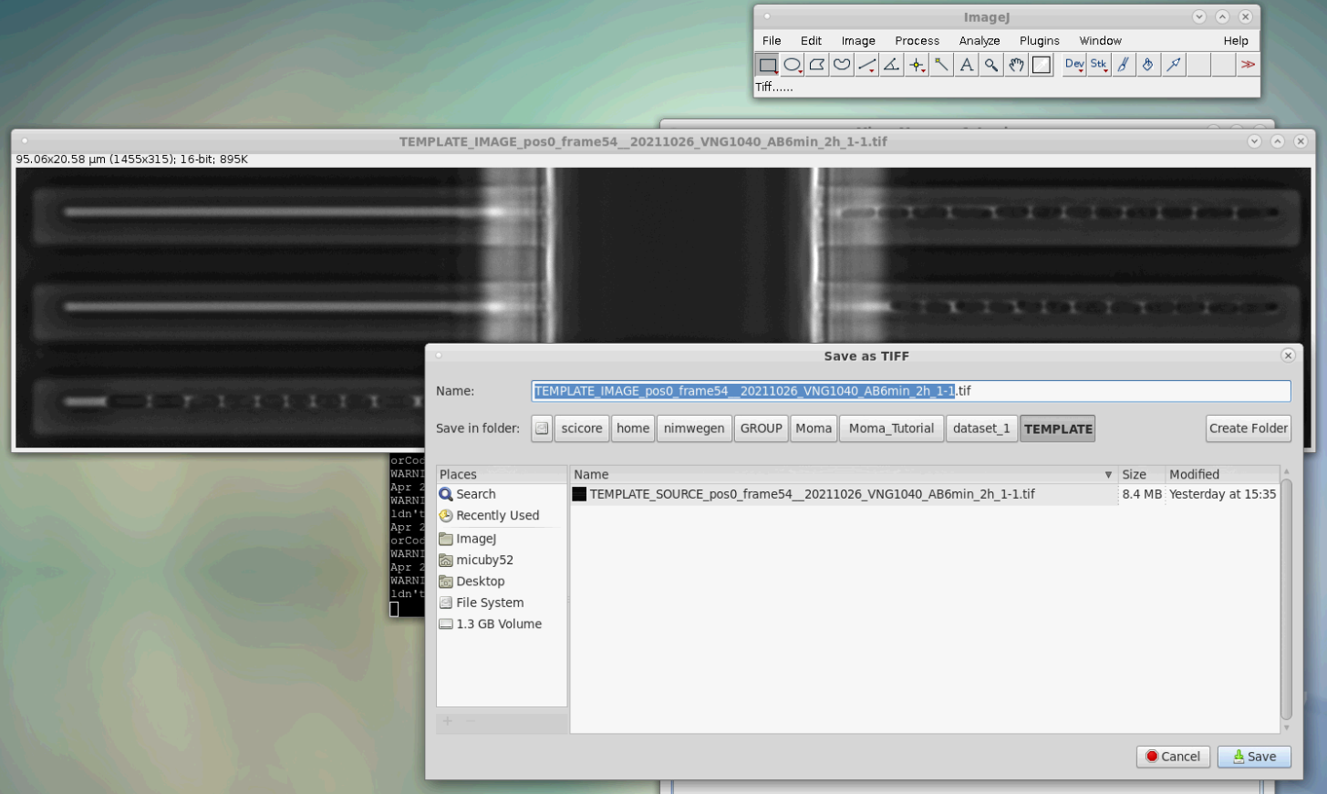
Step 1: Open the image rotation dialog. Step 2: Enable Preview and select Bicubic interpolation. Rotate the image in negative direction so that the main channel of the mother machine is in vertical direction. You can adjust the number of Grid Lines to aid you in aligning the main channel. The rotation angle must be precise to within 0.1 degrees (in the example it is -90.0). Press 'OK', when done. Step 3: Activate the rectangular selection tool in the ImageJ window and drag a rectangle selection on the rotated image, to select the region for the template image. Step 4: Hit Ctrl+Shift+X to crop the image to the selected region and save it. Do not overwrite the template source image. It is still needed for measuring the distance between GLs (see below). 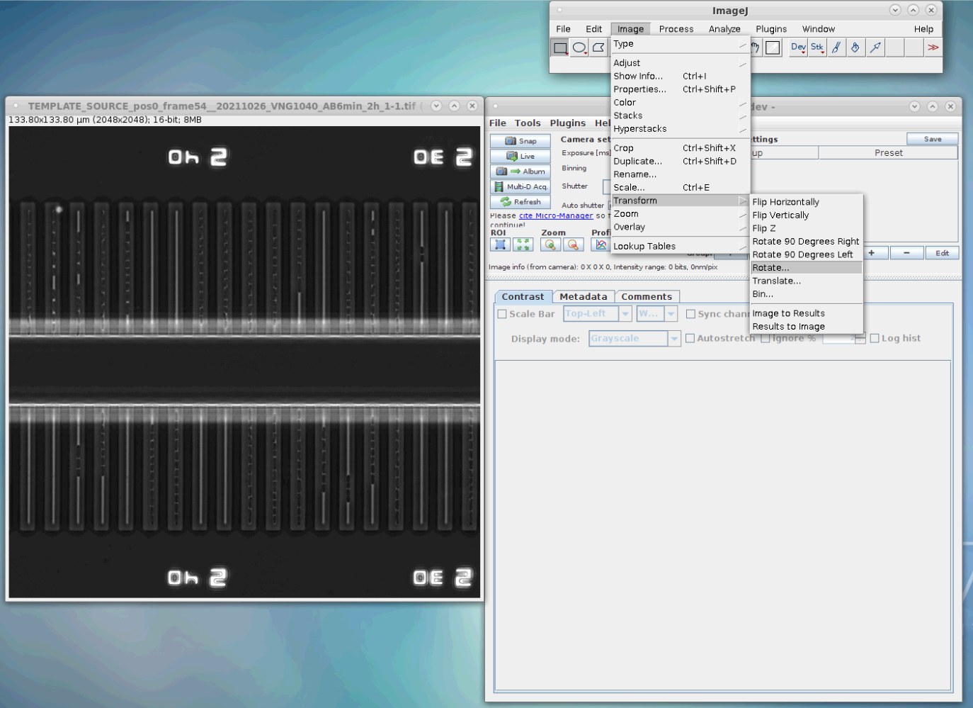


This section explains how create a template configuration file. The template configuration is a JSON file, which specifies where GLs are located in the template image. You can find more information about its parameters here. The reference file is located here:
<ANALYSIS_DIRECTORY>/TEMPLATE/template_config.jsonTo generate a template configuration file follow these steps:
-
Create a new config file in your template folder and copy the following to it:
{
  "description": "",
  "gl_regions": [
    {
      "first_gl_position_from_top": ,
      "gl_spacing_vertical": ,
      "horizontal_range": [
        ,

      ],
        "gl_exit_orientation": ""
    },
    {
      "first_gl_position_from_top": ,
      "gl_spacing_vertical": ,
      "horizontal_range": [
        ,

      ],
        "gl_exit_orientation": ""
    }
  ],
  "name": "",
  "pixel_size_micron": 1.0,
  "template_image_path": ""
}
It should look like this:
Step: Paste the empty configuration from above to start
work on the template configuration.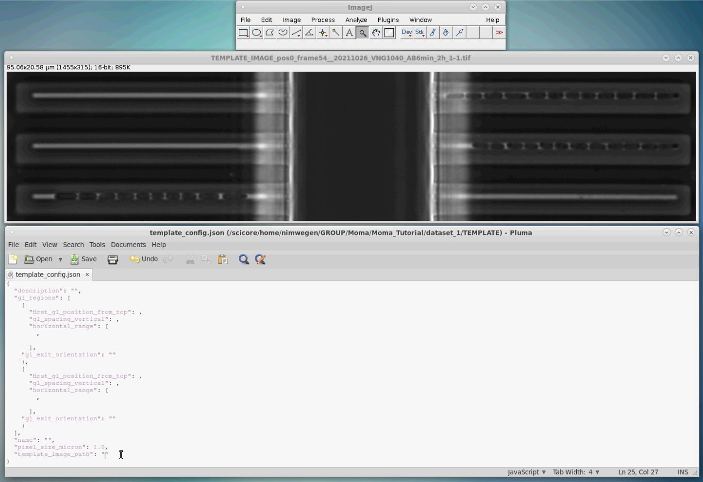
-
Add the path to the template image from above in the field template_image_path:
Step: Add the path to the template image. 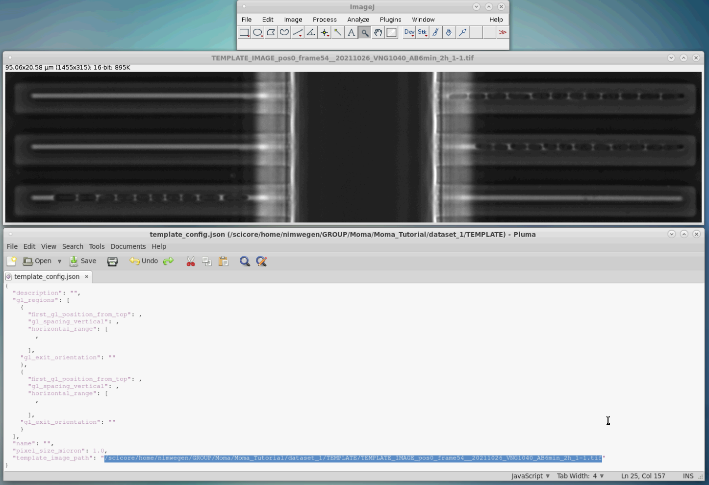
-
Measure the distance between GLs in the template source image and enter it into the template configuration:
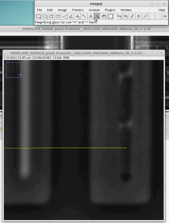
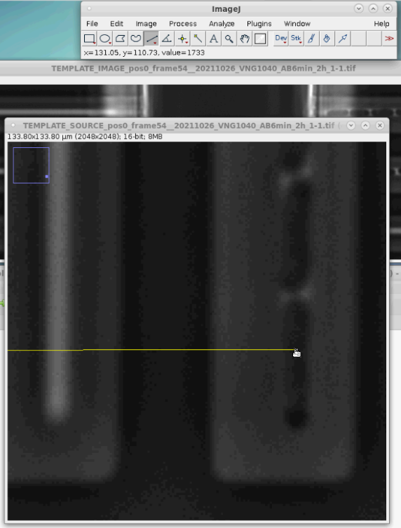
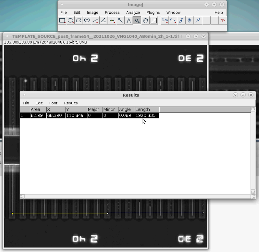
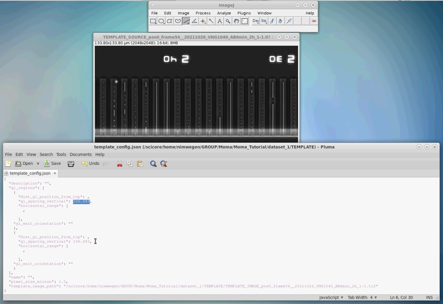
Step 1: Open the template source image and activate the line selection tool in the ImageJ window. Step 2: Draw a line selection from the first to the last GL in the image. Step 3: Refine start and endpoints of the line so that they are centered on their respective GL. This requires switching in the ImageJ window between the Zoom tool (zoom in: left mouse-click; zoom out: right mouse-click) and the line selection tool for adjustments (hover over an end-point and drag it with the left mouse-button). Step 4: Measure the line length in pixels by hitting Ctrl+Shift+M (in this case it is 1920.3). Step 5: Calculate average space between the GLs by dividing the previous value by the number of spaces between GLs spanned by the line. Enter the value into the field gl_spacing_vertical for both gl_regions. In this case: 1920.3/18=106.683 (keep 3 decimals for sufficient precision) 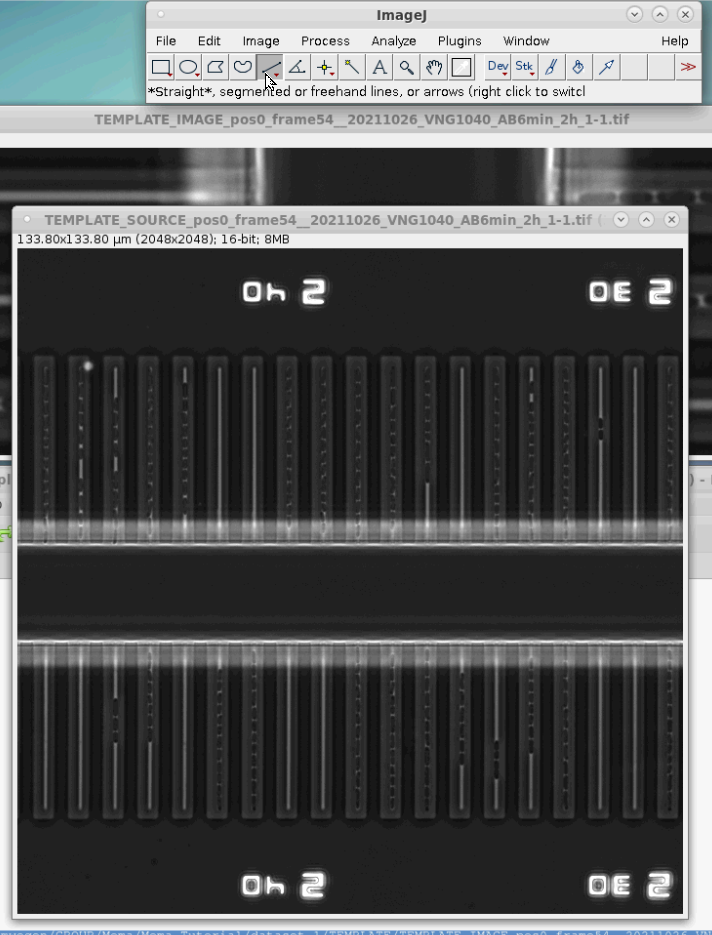
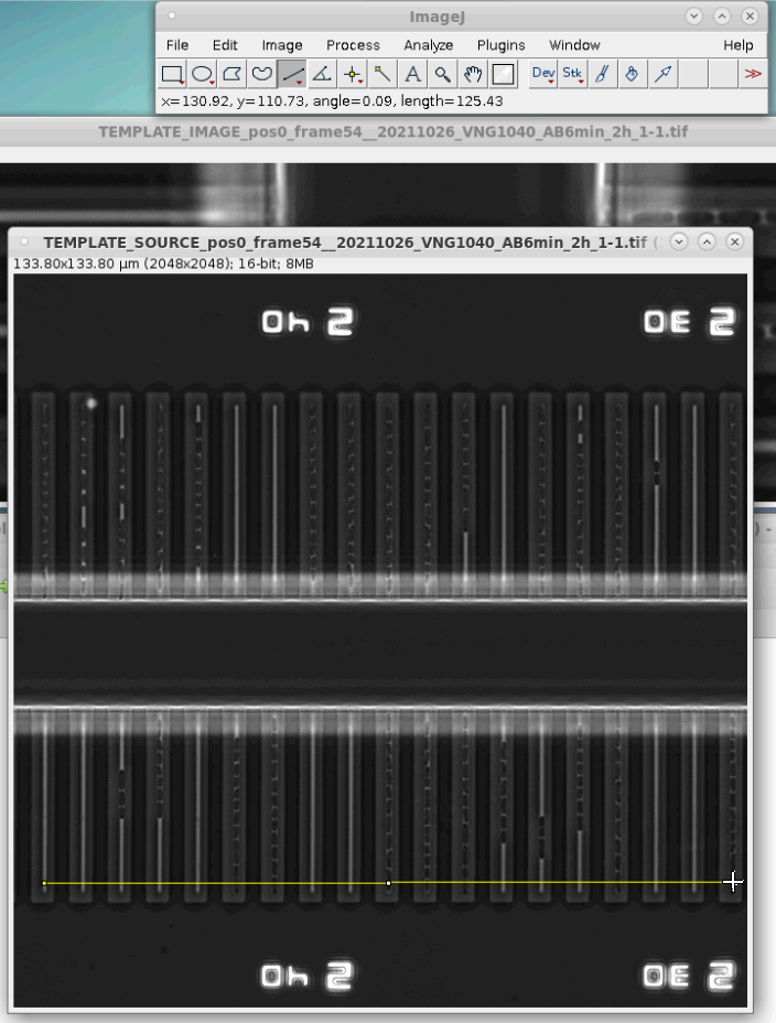
start point: 
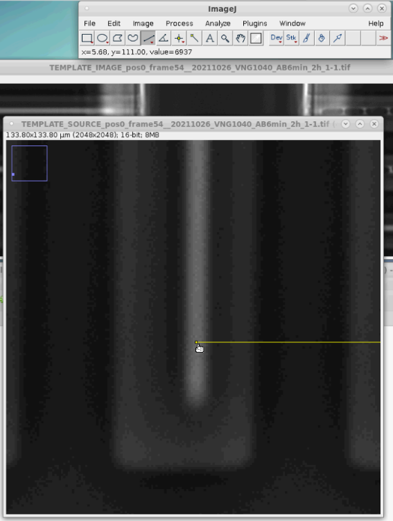
end point:
-
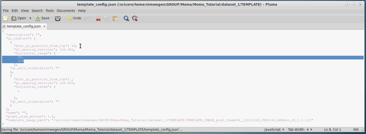
Measure the values of first_gl_position_from_top and horizontal_range for the left gl_region and add them to the template configuration. This is done by locating the cursor at the respective position, while holding the Alt-key. By holding the Alt-key ImageJ will report the cursor position in pixels in the ImageJ window.
Important: Leave a margin of at least 20 pixel at the closed end of the GL (i.e. beyond the last possible position of the mother cell). This is needed for the U-Net model to perform well when segmenting mother cells.Step 1: Measure y-position for first_gl_position_from_top by locating the cursor at the center of the top-left GL. Here the value is: 49 Step 2: Measure first/start x-position for horizontal_range by locating the cursor at the left end GL, leaving a ~20 pixel margin. Here the value is: 32 Step 3: Measure last/end x-position for horizontal_range by locating the cursor at the right end GL outside the hallow. Here the value is: 618 Step 4: Enter the values into the config file. 


-
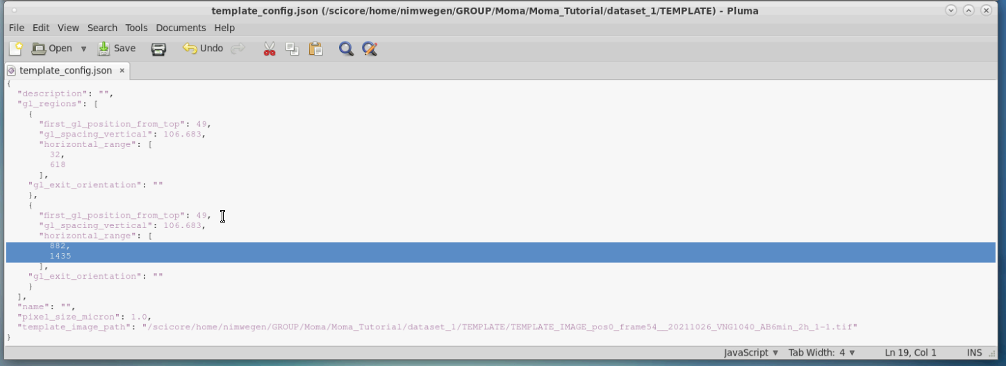
Repeat the previous steps for the second/right gl_region:
Step 1: Measure x-position for first_gl_position_from_top by locating the cursor at the center of the top-left GL. Here the value is: 49 Step 2: Measure first/start x-position for horizontal_range by locating the cursor at the left end GL outside the hallow. Here the value is: 882 Step 3: Measure last/end x-position for horizontal_range by locating the cursor at the right end GL, leaving a ~20pixel margin. Here the value is: 1435 Step 4: Enter the values into the config file. 


-
Set the orientation of the GL exits for both gl_regions in gl_exit_orientation. In the left region the GLs open towards the right so we set gl_exit_orientation to right. For the right region they open towards the left, so we set gl_exit_orientation to left.
Step 1: Enter values for gl_exit_orientation. 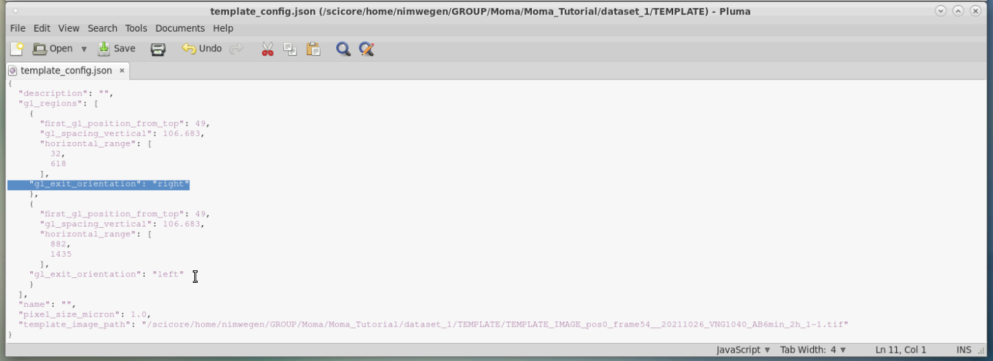
To create the bash script, we start from this template:
#!/bin/bash

PREPROC_DIR_TPL=""
RAW_PATH=""
FLATFIELD_PATH=""

POS_NAMES=()

GL_DETECTION_TEMPLATE_PATH=""
ROTATION=

IMAGE_REGISTRATION_METHOD=1
FRAMES_TO_IGNORE=()

NORMALIZATION_CONFIG_PATH="true"
NORMALIZATION_REGION_OFFSET=120

#### DO NOT EDIT BELOW THIS LINE ####
ROI_BOUNDARY_OFFSET_AT_MOTHER_CELL=0

# generate an array of same length as position array, with every element containing the ROTATION scalar value
ROTATIONS=$ROTATION
for f in `seq ${#POS_NAMES[*]}`
do
        f=`echo $f - 1 | bc`
        ROTATIONS[$f]=$ROTATION
done

source mm_dispatch_preprocessing.sh
mm_dispatch_preprocessing
We adapt the template in order to process positions Pos1 and Pos7 of the experiment and save the preprocessed data to the folder:
<ANALYSIS_DIRECTORY>/preprocessed_dataThis is the adapted bash-script (located at <ANALYSIS_DIRECTORY>/process_positions.sh):
#!/bin/bash

PREPROC_DIR_TPL="<ANALYSIS_DIRECTORY>/preprocessed_data/mmpreproc_%s/"
RAW_PATH="<PATH_TO_FIRST_OME_TIF_MEASUREMENT_FILE>"
FLATFIELD_PATH="<PATH_TO_FIRST_OME_TIF_FLATFIELD_FILE>"

GL_DETECTION_TEMPLATE_PATH="<ANALYSIS_DIRECTORY>/TEMPLATE/template_config.json"

POS_NAMES=(Pos0 Pos7)

TMAX=5

ROTATION=90.0

IMAGE_REGISTRATION_METHOD=1
FRAMES_TO_IGNORE=()

NORMALIZATION_CONFIG_PATH="true"
NORMALIZATION_REGION_OFFSET=120

#### DO NOT EDIT BELOW THIS LINE ####
ROI_BOUNDARY_OFFSET_AT_MOTHER_CELL=0

# generate an array of same length as position array, with every element containing the ROTATION scalar value
ROTATIONS=$ROTATION
for f in `seq ${#POS_NAMES[*]}`
do
        f=`echo $f - 1 | bc`
        ROTATIONS[$f]=$ROTATION
done

source mm_dispatch_preprocessing.sh
mm_dispatch_preprocessing
The parameters that were changed/added above are (an explanation of all parameters can be found here):
-
PREPROC_DIR_TPL: Path to the output folder where the preprocessed data will be stored.
Important: You have to append "/mmpreproc_%s/" to the desired output folder. This is for legacy reasons. -
RAW_PATH: Path to the first TIFF-file of the OME-TIFF stack.
-
FLATFIELD_PATH: Path to the first TIFF-file in the OME-TIFF stack containing the corresponding flat-field images.
-
GL_DETECTION_TEMPLATE_PATH: This is the path to the template configuration file, that we created earlier.
-
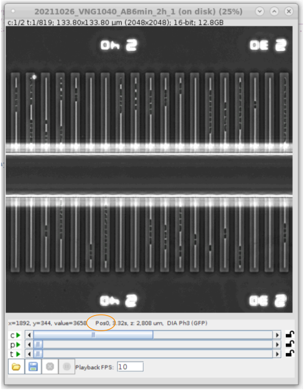
POS_NAMES: This array defines that names of the positions in the OME-TIFF stack that will be processed. The name of a position can be obtained from MicroManager:
-
TMAX: Setting this value to 5 preprocesses only the first 5 frames of the experiment. This is useful for testing the preprocessing script before running the actual preprocessing or if there were experimental issues at later time points that you want to ignore. Once you are confident that the configuration works as expected, comment this value out (e.g. by adding a #, so: #TMAX=5) or set it to the desired value.
-
ROTATION: This is the rotation angle of the image that was determine in the section Generating the template image.
Important: You have to enter the negative value of the angle reported by ImageJ, because ImageJ uses a different convention for the rotation angle than the preprocessing code. Hence we enter 90.0 instead of the -90.0 that we determined before.
For an explanation of the remaining parameters please see here.
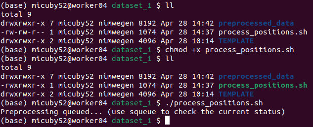
Open a terminal window and navigate to the location of the bash script.
If you created a new file from scratch you will have to first make it
executable using the command chmod. Then launch it:
You can monitor the progress of the preprocessing of each position by running:
watch -n1 'squeue -u $USER'Which gives output like this:

Here will give an overview of the data that the preprocessing outputs. It located here:
<ANALYSIS_DIRECTORY>/preprocessed_dataThis is a screenshot of that folder:
| Overview of the preprocessing output |
|---|
 |
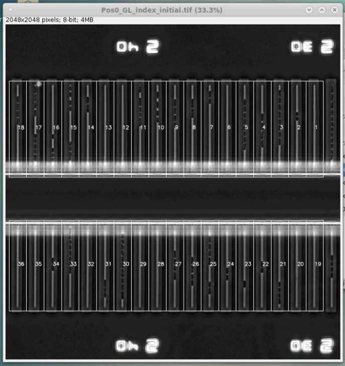
The index images *_GL_index_initial.tif and *_GL_index_final.tif indicate the GL ROIs that were detected and stored. They show their bounding boxes overlaid on the first and last frames of the processed frame range:
| Screenshot of initial GL ROI index image showing first frame with overlays. |
Screenshot of final GL ROI index image showing last frame with overlays. |
|---|---|
 |
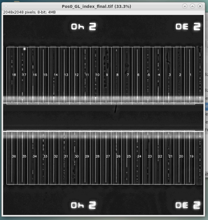 |
Important: GL ROIs are only stored if they lie inside the full frame image for all time steps. GL ROIs that (partially) move outside of the full frame due to image drift/shift are discarded (this can happen in particular for GLs located at the image border).
The GL ROIs of each position are stored in the folders Pos* in separate GL subfolders:
| Content of the Pos0 folder. |
|---|
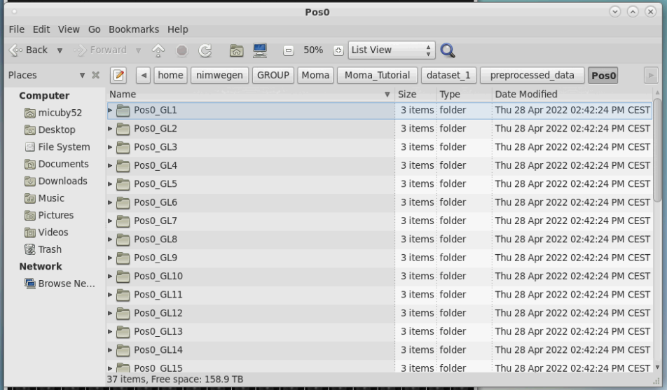 |
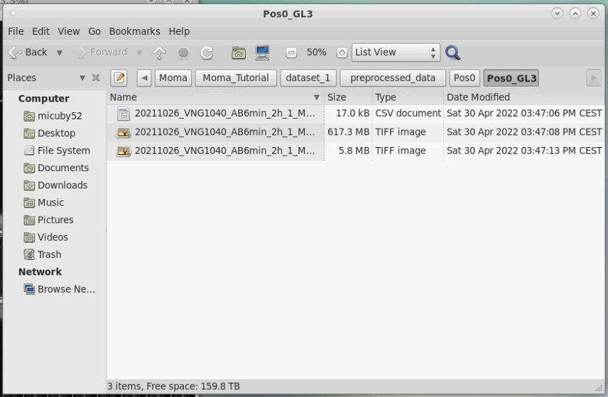
Each GL folder contains three files:
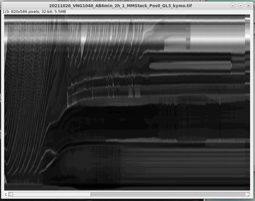
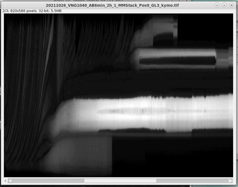
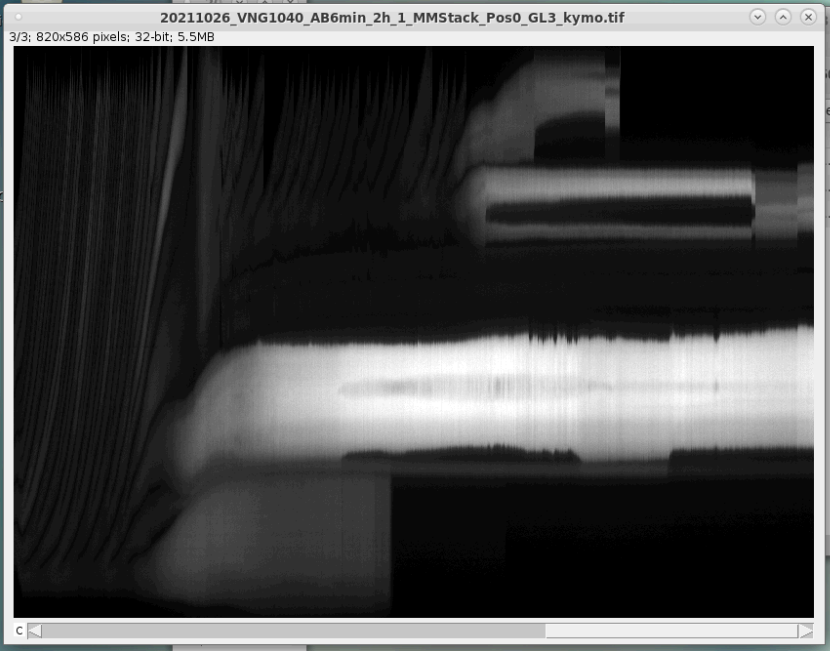
| Example folder content for GL3 of Pos0: The minimum and maximum values used for normalization are stored in: 20211026_VNG1040_AB6min_2h_1_MMStack_Pos0_GL3.csv A kymograph of the GL vertical center line is stored in: 20211026_VNG1040_AB6min_2h_1_MMStack_Pos0_GL3_kymo.tif The GL ROI is contained in: 20211026_VNG1040_AB6min_2h_1_MMStack_Pos0_GL3.tif | Screenshots of the first frame in the GL ROI stack. Each FL channel in the input image is output twice: The first duplicate is the flatfield-corrected signal; the second is the unaltered signal. | Screenshots of PhC (left) and FL (right) kymograph images. Again the FL channel is duplicated for the flat-field correct and non-corrected signal. |
|---|---|---|
 |
  
|
|
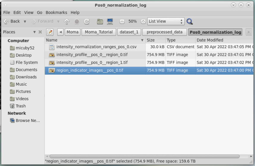
During preprocessing the input images are normalized. Information on the normalization can be found in the respective normalization log-folder of each position:
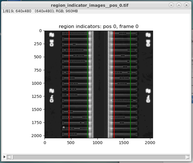
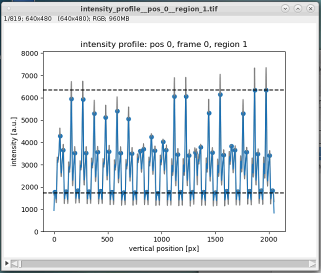
| Screenshot of the normalization log folder of Pos0. | Screenshot of region_indicator_images__pos_0.tif. These images indicate the regions, which were used for the normalization of each GL region (red: start of horizontal region; green: end of horizontal region). These images can also helpful for checking if the image registration (i.e. compensating image drift) worked correctly. If so, the positions of the GLs should not change between frames. | Screenshots of intensity_profile__pos_0__region_0.tif and intensity_profile__pos_0__region_1.tif. These image show the intensity profile that was obtained from the normalization regions in region_indicator_images__pos_0.tif. They help in debugging problems with the intensity normalization. |
|---|---|---|
 |
 |
|
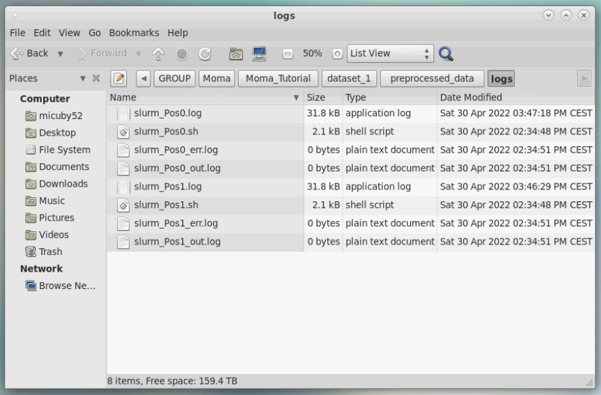
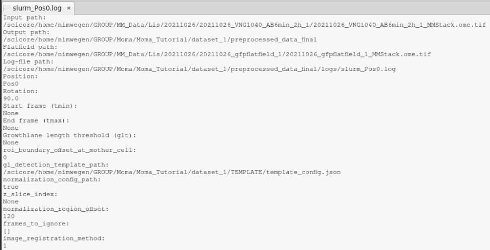
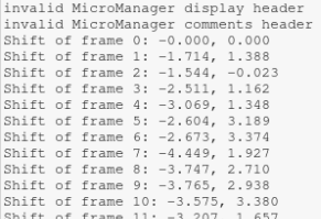
The files in the log folder are intended for debugging. For example, the bash-script slurm_Pos0.sh is the script was run to process Pos0. The slurm_Pos0.log contains the log-output from that bash-script.
| Content of the log folder. | Content of slurm_Pos0.log. It contains information on the preprocessing settings and the shift that was measured during image registration. |
|---|---|
 |
|